FEATURED-RESEARCH MEDIA
ENGLISH VERSIONS BELOW
http://rcqt.science.cmu.ac.th/wp-content/uploads/2026/01Black-scholes equation in quantitative finance – Eng.png
Executive Summary
The traditional Black–Scholes–Merton model, while foundational to modern quantitative finance, is increasingly viewed as inadequate due to its reliance on static assumptions—specifically constant volatility, risk-free interest rates, and dividend yields. This document synthesizes research proposing a generalized Black–Scholes equation (BSE) that incorporates time-varying and state-dependent parameters governed by power-law dynamics.By utilizing variable transformations and Laplace transforms, researchers have successfully mapped the generalized BSE to a generalized Schrödinger equation from quantum mechanics. A critical finding of this synthesis is the emergence of “position-dependent mass” (PDM) within the financial context, where market variables are modeled via wave-like dynamics. This interdisciplinary approach provides a more robust framework for pricing derivatives, explaining market irregularities, and aligning theoretical models with empirical data such as high-frequency stock returns and “fat-tail” distributions.
Limitations of the Traditional Black–Scholes–Merton Model
The standard Black–Scholes model is used to estimate the fair price of European options, but it operates under several restrictive and often unrealistic hypotheses:
● Constant Parameters: It assumes volatility ( $\sigma$ ), risk-free interest rates ( $r$ ), and dividend yields ( $D$ ) remain constant over the life of the option.
● Lognormal Distribution: It assumes a stationary lognormal distribution for stock prices, which fails to account for large price fluctuations observed in real-world markets.
● Frictionless Markets: The model ignores transaction costs and assumes a perfectly liquid market.
● Time-Invariance: It fails to reflect the dynamic nature of risk and investor expectations, particularly during periods of structural shifts or market turbulence.
The Generalized Black–Scholes Equation with Variable Parameters
To address the shortcomings of the traditional model, recent research introduces time-varying parameters governed by power laws. This aligns the model with empirical evidence suggesting that parameters like volatility and asset prices obey power-law functions.
Mathematical Framework
The generalized BSE for European options with time-varying parameters is expressed as: $$\frac{\partial V}{\partial t} = (r(t) – D(t))S \frac{\partial V}{\partial S} + \frac{1}{2}\sigma^2(t)S^2 \frac{\partial^2 V}{\partial S^2} – r(t)V$$Where:
● $\sigma^2(t)$ : Time-dependent volatility.
● $r(t)$ : Time-dependent risk-free interest rate.
● $D(t)$ : Time-dependent dividend payout.
Power-Law Dynamics
The model assumes that these parameters follow power-law functions, such as:
● $\sigma^2(t) = \sigma^2_0 t^{\beta-1}$
● $r(t) = r_0 + r_1 t^{\beta-1}$
● $D(t) = D_0 + D_1 t^{\beta-1}$These power laws are effective in explaining the “tail distributions” of trades and returns, as the power-law property of investor assets is often inherited by these market processes.
Quantum Finance: The Path to the Schrödinger Equation
A significant advancement in this field is the established analogy between the Black–Scholes evolution equation and the Schrödinger equation of quantum mechanics.
The Black–Scholes–Schrödinger Connection
By identifying the option price as a “state function” (wave function $\psi$ ), the evolution of financial instruments can be understood through quantum dynamics. The research demonstrates that:
● Effective Hamiltonian: The generalized BSE can be converted into an effective quantum Hermitian Hamiltonian ( $H_{eff}$ ).
● Wave-Particle Duality: Stock prices exhibit corpuscular properties (traded at specific prices) while their fluctuations exhibit wave-like behavior.
● Position-Dependent Mass (PDM): Under specific constraints, the generalized BSE leads to a Schrödinger equation characterized by PDM. In this context, “mass” may refer to the “mass of the stock” or the “capital input” into the system.
Emergent Phenomena
● Wick Rotation: The use of Wick rotation ( $t = -i\tau$ ) ensures genuine solutions and maps the initial option price to a quantum state, allowing for the simulation of time-dependence in imaginary time space.
● Singular Wave Solutions: Under certain assumptions, resulting quantum wave solutions are comparable to lump and solitary waves found in nonlinear sciences, potentially explaining rare market events.
Methodological Comparison in Financial Literature
Various analytical and numerical techniques have been developed to solve the generalized BSE. The following table summarizes key approaches:| Methodology | Key Contribution / Tool || —— | —— || Lie Algebraic Approach | Propagator techniques for time-dependent parameters. || Malliavin Calculus | Sets up analytic formulas for small volatility. || Fractional Calculus | Incorporates “memory effects” to estimate large price fluctuations. || Laplace Transform | Solves diffusion equations and allows for stability analysis. || Neural Networks (AI) | Processes complex financial data for market price estimation (e.g., Physics-Informed Neural Networks). || Monte Carlo Simulation | Ideal for path-dependent payoffs and variable volatility. || Quantum Algorithms | Estimates costs of Asian and barrier options under Heston stochastic volatility models. |
Key Findings and Observations
The analysis of the generalized model with variable parameters yields several critical insights into option price behavior:
● Time Sensitivity: Option prices generally decrease as time passes and expiration approaches. Conversely, the value of a call option increases as the time to expiration increases.
● Asymptotic Limits: The option price reaches an asymptotic limit after a specific period of evolution.
● Parameter Influence ( $\beta$ and $\alpha$ ): Numerical simulations indicate that option prices are highly sensitive to power-law parameters. Option prices generally increase with a decreasing $\beta$ parameter.
● Market Liquidity: Quantum Hamiltonians become “local” when the profit/loss ratio is small compared to trading turnover, a result that may describe the high liquidity required for efficient markets.
● Real-World Alignment: By allowing parameters to evolve according to empirically supported power laws, the generalized model aligns more closely with observed market data than the static Black–Scholes model.
Conclusion
The integration of tools from mathematical physics—specifically the Schrödinger equation and PDM formalism—into financial economics represents a forward-thinking shift in quantitative finance. This approach addresses the long-standing limitations of the traditional Black–Scholes framework by providing a robust, flexible system capable of capturing the complexities, irregularities, and dynamic risks of contemporary global markets.
http://rcqt.science.cmu.ac.th/wp-content/uploads/2026/02Acceleration-Dependent Hamiltonian – Eng.png
Executive Summary
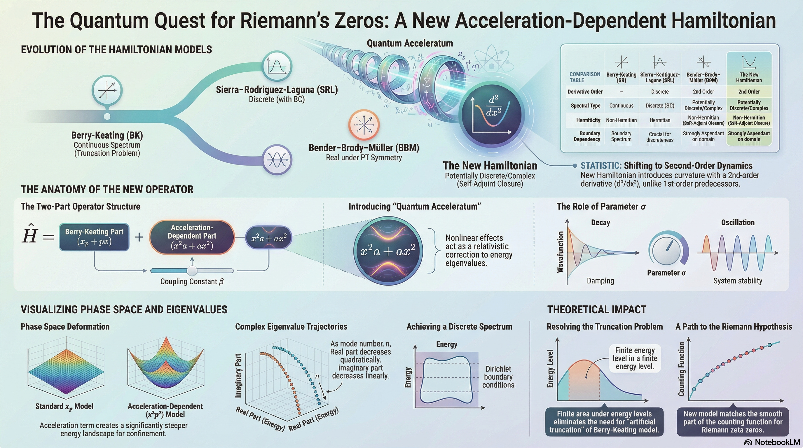
The provided research introduces a novel acceleration-dependent Hamiltonian operator ( $\hat{H}$ ) designed to investigate the spectral properties of the zeros of the Riemann zeta function. This operator synthesizes the established Berry-Keating operator with a new “quantum acceleratum operator,” introducing nonlinear effects beyond conventional canonical mechanics. The central objective is to provide a mathematical framework that supports the Hilbert-Polya conjecture, which suggests that the non-trivial zeros of the Riemann zeta function correspond to the eigenvalues of a Hermitian operator.
Critical takeaways include:
● Operator Composition: The new Hamiltonian is a second-order differential operator that combines linear dilation (from the Berry-Keating model) with higher-order interactions involving position and acceleration.
● Spectral Discreteness: While the standard Berry-Keating model yields a continuous spectrum, the new operator can support a discrete spectrum under specific boundary conditions or domain constraints, a necessary requirement for modeling the discrete zeros of the Riemann function.
● Physical Realizability: By incorporating acceleration-dependent terms, the model introduces relativistic-like corrections that can bound classical trajectories, potentially resolving the “truncation problem” found in previous models.
● Hybrid Framework: The operator is characterized as a hybrid, utilizing the real-structure of the Sierra–Rodríguez-Laguna model and the complex deformation characteristic of the Bender–Brody–Müller Hamiltonian.
1. Context: The Riemann Hypothesis and the Hilbert-Polya Conjecture
The Riemann zeta function $\zeta(s)$ is a function of a complex variable $s = \sigma + it$ . The Riemann hypothesis states that all non-trivial zeros of this function lie on the critical line $Re(s) = 1/2$ .
1.1 The Hilbert-Polya Conjecture
The Hilbert-Polya conjecture posits that the imaginary parts of these zeros ( $n_t$ ) correspond to the eigenvalues of a Hermitian (self-adjoint) operator. If such an operator is identified, the $n_t$ values must be real, thereby proving the Riemann hypothesis. To satisfy the conjecture, a candidate Hamiltonian must meet three criteria:
Chaos: It must be chaotic in the classical regime with isolated periodic orbits related to prime numbers.
Broken Symmetry: It must break time-reversal symmetry to align with the Montgomery-Odlyzko Gaussian Unitary Ensemble of Random Matrix Theory.
Dimensionality: It must be quasi-one dimensional.
1.2 Limitations of Previous Models
The document identifies several existing Hamiltonian candidates and their inherent flaws:
● Berry-Keating ( $\hat{H} = xp$ ): Suffers from a “truncation problem” because it requires artificial bounds to produce a discrete spectrum; additionally, prime numbers do not appear in its periodic orbits.
● Sierra and Rodriguez-Laguna ( $H_{S-RL}$ ): Addresses the truncation problem but requires specific potentials or boundary conditions for discreteness.
● Bender–Brody–Müller ( $\hat{H}_{BBM}$ ): Promising but non-Hermitian and involves non-local operators, making physical connection difficult.
2. The Acceleration-Dependent Hamiltonian Operator
The research introduces a new Hamiltonian $\hat{H}$ based on the notion of a “quantum acceleratum operator” ( $\hat{a}$ ). This is motivated by findings in maximal acceleration and nonlocal-in-time kinetic energy.
2.1 Mathematical Structure
The operator consists of two independent parts:
Berry-Keating Part: $\hat{H}_{BK} = \frac{1}{2}(xp + px)$ .
Acceleratum Part: $\hat{H}_a \propto \frac{1}{2}(x^2 a + ax^2)$ , where $\hat{a}$ is the acceleratum operator.The resulting second-order differential Hamiltonian is expressed as: $$\hat{H} = -\sigma x^2 \frac{d^2}{dx^2} + (-i – 2\sigma)x \frac{d}{dx} + \frac{-i – 2\sigma}{2}$$ Where:
● $\sigma = \beta – \alpha$ is a parameter determined by coupling constants.
● The operator introduces curvature into the phase space, reminiscent of deformations used to generate discrete spectra.
2.2 Comparative Analysis of Models
The following table summarizes the features of the new Hamiltonian compared to its predecessors:| Feature | Berry–Keating | Sierra–Rodríguez-Laguna | Bender–Brody–Müller | The New Hamiltonian || —— | —— | —— | —— | —— || Operator Type | Linear dilation $xd/dx$ | Quadratic + linear derivatives | Complexified dilation | 2nd Order Derivative (Hybrid structure) || Spectral Type | Continuous | Can be discrete with BC | Discrete/complex | BC-dependent; potentially discrete/complex || Boundary Conditions (BC) | Optional for continuum | Crucial for discreteness | Crucial for PT-symmetry | Crucial; determines spectrum and reality || Hermiticity | Hermitian | Hermitian | Non-Hermitian / PT-symmetric | Non-Hermitian (standard $L^2$ sense) || Key Novelty | Simple semiclassical | Discrete spectrum | Complex deformation | Hybrid: SR structure + BBM complexification |
3. Spectral Properties and Self-Adjointness
The study performs a deep analysis of the spectral nature of the new operator, emphasizing that discreteness is a “key indicator of physical stability.”
3.1 Conditions for Hermiticity
The operator is found to be self-adjoint or Hermitian under specific assumptions (e.g., $\sigma \in \mathbb{R}$ ). However, the document notes that because the operator contains complex terms, it is non-Hermitian in the standard $L^2(\mathbb{R})$ sense. Its spectral reality depends heavily on the chosen domain and boundary conditions.
3.2 Spectral Discreteness vs. Continuity
Continuous Spectrum: On the whole half-line $[0, \infty)$ , the operator typically yields a continuous spectrum. In the “natural Hilbert space unitary picture,” the operator becomes a constant-coefficient differential operator on a non-compact domain, forcing a continuous range of eigenvalues.
Discrete Spectrum: Discretization is achieved through:
Imposing boundary conditions (e.g., Dirichlet) on a finite domain $\epsilon, R$ .
Introducing a confining potential.
Periodic compactification (working on a multiplicative circle).
Eigenvalue Trajectories: As the mode number $n$ increases, the real part of the eigenvalues decreases quadratically, while the imaginary part decreases linearly.
4. Classical and Relativistic Perspectives
The document distinguishes between the behavior of the system at different “levels” of interaction.
4.1 Classical Level
At the classical level, the acceleratum is negligible. The Hamiltonian reduces to the Berry-Keating form ( $H \approx xp$ ).
● Trajectories: Uniformly unstable; trajectories tend away from the origin.
● Spectrum: Continuous due to unbounded trajectories.
● Counting Function: For specific parameters ( $4\beta = \alpha\pi$ ), the model approximates the smooth part of the counting function for the non-trivial zeros of the Riemann zeta function.
4.2 Relativistic Level
At this level, the acceleratum becomes dominant ( $H \propto x^2 a$ ).
● Boundedness: Unlike the Berry-Keating model, the trajectories are naturally bounded ( $p = 1 + \beta – \beta x^2$ ).
● Implication: The spectrum is discrete and can be compared directly with the discrete zeros of the Riemann zeta function without the need for artificial truncation of the phase space.
5. Conclusion and Future Research
The introduction of acceleration-dependent terms offers a rigorous foundation for future exploration of Berry-Keating-type Hamiltonians. The research demonstrates that higher-order operator interactions can restore discreteness in systems otherwise governed by scaling invariance.
Key conclusions include:
● The interplay between the dilation operator and the acceleration coupling determines the transition from continuous modes to localized, normalizable eigenstates.
● The acceleratum operator effectively generates a restoring force analogous to harmonic confinement.
● Future work is required to explore explicit realizations of the operator $\hat{a}$ and analyze higher-order polynomial deformations to further refine the connection to the Riemann zeros.
A FRACTAL ELECTROCHEMICAL POROUS MODEL FOR LITHIUM-ION BATTERIES
http://rcqt.science.cmu.ac.th/wp-content/uploads/2026/03A fractal electrochemical porous – Eng.png
Executive Summary
This briefing document synthesizes the findings of a 2026 study published in the Journal of Energy Storage regarding a novel fractal electrochemical model for lithium-ion batteries (LIBs). The research introduces a “product-like fractal measure” to analyze complex dynamics within porous media, specifically focusing on the secondary particles of LIBs.The study demonstrates that incorporating fractal dimensions ( $\alpha$ ) into electrochemical modeling offers significant advantages over classical Euclidean models.
Key findings include:
● Enhanced Ion Transport: Lower fractal dimensions lead to increased lithium-ion ( $Li^+$ ) salt concentrations at interfaces, improving cation-solvent interactions and reducing internal resistance.
● Rapid Equilibrium: Systems with fractal structures reach steady-state concentration faster than smooth surfaces, suppressing polarization and enabling stable operation under high C-rates.
● Dendrite Suppression: The model reveals that in fractal dimensions, lithium dendrites grow insignificantly over time. Current density becomes more uniform, and dendrite tips lose their status as preferred deposition sites, offering a potential solution to internal short circuits.
● Structural Optimization: Fractal geometries promote a more homogeneous ion distribution and minimize internal mechanical stresses, directly extending the operational lifetime of battery components.
1. Introduction to the Fractal Approach
Standard electrochemical models often struggle to capture the multiscale effects of mass transport within the complex, anisotropic porous microstructures of LIB electrodes. This study utilizes the Li and Ostoja-Starzewski (LOSA) approach, which describes dynamics in anisotropic media through fractal spatial dimensions.
Core Motivations for Fractal Modeling
● Surface-to-Volume Optimization: Fractal electrodes can minimize internal resistance while maximizing the active surface area.
● Anisotropic Media: LOSA is particularly effective for systems where fractal dimensions vary in different directions, such as the secondary particles composed of fine primary particles and binders.
● Safety and Performance: Traditional models face challenges with non-uniform power distribution and “plating” risks; fractal structures mitigate these by ensuring more uniform current and ion distribution.
2. The Electrochemical Model in Fractal Dimensions
The study derives a modified electrochemical model by embedding fractal structures into classic transport equations. This includes terms for ion diffusion, electrolyte conductivity, and reaction surface area.
Key Evolution Equations
The model consists of four primary partial differential equations governing:
Electric Potential in the Electrolyte: Accounts for effective conductivity ( $\kappa$ ) and transference numbers.
Electric Potential in the Solid Phase: Incorporates solid-phase conductivity ( $\sigma_S$ ).
Lithium Concentration in the Electrolyte: Uses variable porosity ( $\epsilon(R)$ ) and a variable effective diffusion coefficient ( $D_l$ ).
Lithium Concentration in Primary Particles: Follows a modified Fick’s second law in fractal dimensions.
Physical Parameters Used for Simulation
The following table outlines the representative numerical values applied in the Matlab-based computational analysis:| Parameter | Symbol | Value || —— | —— | —— || Temperature | $T$ | $35^\circ$ C || Faraday Constant | $F$ | 13.901 C/g || Porosity Constant | $\epsilon_0$ | 25% || Effective Electrolyte Conductivity | $\kappa$ | 0.0975 S/cm || Solid Diffusion Coefficient | $D_s$ | $10^{-14}$ m²/s || Maximum Solid $Li^+$ Concentration | $C_{s,max}$ | 51,830 mol/m³ || Particle Radius (Secondary) | $R_s$ | $10^{-5}$ m |
3. Analysis of $Li^+$ Concentration Dynamics
The degree of the fractal dimension ( $\alpha$ ) is the primary factor determining the total $Li^+$ concentration and distribution efficiency.
Impact of Lower Fractal Dimensions ( $\alpha < 1$ )
● Increased Salt Concentration: For values where $\alpha \ll 1$ , the concentration of lithium salt reaches significantly higher levels than in the ideal Euclidean case ( $\alpha = 1$ ). This improves ion transport properties and battery safety.
● Interface Stabilization: Elevated concentrations at the interface facilitate the formation of a lithium-rich solid electrolyte interphase (SEI) with high ionic conductivity.
● Reduced Concentration Polarization: A larger reservoir of ions at the electrode surface reduces the lag between ion transport and electrochemical reactions, preventing sudden voltage drops.
Temporal and Spatial Equilibrium
The model demonstrates that fractal geometry ( $1/2 < \alpha \le 1$ ) leads to a faster attainment of steady-state concentration.
● Mechanical Integrity: Rapid equilibration prevents temporal concentration gradients that cause heterogeneous expansion/contraction, thereby reducing cracking and loss of active material.
● High C-rate Support: Early stabilization of interfacial $Li^+$ concentration allows for more efficient fast-charging and deep-discharging performance.
4. Dendrite Mitigation and Current Density
Lithium dendrite growth is a critical safety issue, potentially causing internal short circuits and thermal runaway. The fractal model provides a “fresh standpoint” on this problem.
The Dendrite Tip Current Ratio ( $i_t/i_f$ )
The ratio of current density at dendrite tips ( $i_t$ ) to that of a flat surface ( $i_f$ ) is a key indicator of growth probability.
● Uniformity in Fractal Structures: At $\alpha = 0.9$ , the current distribution becomes nearly flat across the particle. This indicates that dendrite tips are not favored sites for deposition compared to smooth surfaces.
● Euclidean Disadvantage: At $\alpha = 1$ , the current distribution is non-uniform, allowing dendrite tips to become active spots, which increases the likelihood of seed formation and growth.
Slower Growth Rates
The study reveals a motivating feature regarding dendrite length ( $h$ ):
● Fractal Stability: As $\alpha$ decreases (moving toward fractal geometry), the slope of dendrite growth over time becomes significantly flatter.
● Suppression Mechanism: The fractal structure enlarges reaction zones and distributes current more uniformly, ensuring that if dendrites do form, they grow at a “too small magnitude” to easily penetrate the separator.
5. Porosity and Structural Observations
The model accounts for variable porosity, which is found to decrease gradually with increasing distance from the particle core, particularly when $\alpha \ll 1$ .
● Electronic Conductivity: Reductions in porosity and porous wall molar flow allow for more active material or conductive additives in the solid phase, resulting in higher electronic conductivity.
● Electrolyte Access: Variable porosity designs can improve discharge capacity by 30% for half-cell configurations and up to 60% for full cells by providing greater electrolyte access without sacrificing power capability.
6. Conclusions and Future Perspectives
The implementation of the product-like fractal measure (LOSA) proves the relevance of fractal dimensions in the electrochemical analysis of lithium-ion batteries.
Strategic Takeaways
● Performance Enhancement: Fractal electrodes offer a potential solution to the dendrite growth problem while simultaneously enhancing $Li^+$ concentration and transport speed.
● Reliability: By reducing internal stresses and promoting homogeneous ion distribution, fractal structures extend the calendar and cycle life of the battery.
● Experimental Direction: The study serves as a guideline for the manufacturing of microscopic structures and the invention of fractal electrodes using microfabrication and nanotechnology.
Future Research Directions
The authors identify several areas for continued investigation:
● Inclusion of temperature effects and liquid-cooled heat dissipation.
● Applying the fractal model to specific battery chemistries, such as LFP (Lithium iron phosphate) and NMC (Nickel Manganese Cobalt).
● Validating the model against real battery data and image-based simulations to determine exact fractal dimensions from physical electrodes.
ACCELERATION IN QUANTUM MECHANICS AND ELECTRIC CHARGE QUANTIZATION: A BRIEFING DOCUMENT
http://rcqt.science.cmu.ac.th/wp-content/uploads/2026/04Acceleration in quantum mechanics – Eng.png
Executive Summary
This document synthesizes the findings of a 2021 study by Rami Ahmad El-Nabulsi and Waranont Anukool regarding the integration of acceleration into the framework of quantum mechanics. By utilizing a Generalized Derivative Operator (GDO), the researchers derived an Extended Schrödinger Equation (ESE) that explicitly incorporates the reduced Compton wavelength of a particle.The study demonstrates that the inclusion of acceleration leads to significant modifications in wave functions and discrete energy levels across various potentials.
Key takeaways include:
● Enhanced Energy States: Ground state energy levels for particles in gravitational and Cornell potentials are significantly higher (“improved”) when acceleration is accounted for compared to standard quantum mechanical models.
● Charge Quantization: The theory provides a mechanism for the quantization of electric charge without the necessity of Dirac monopoles or complex gauge theories, addressing a long-standing puzzle in physics.
● Scale Dependency: The ESE reduces to the standard Schrödinger equation in the limit of large Compton wavelengths or small particle rest masses, but diverges significantly at the quantum scale where acceleration is crucial.
Theoretical Framework: The Generalized Derivative Operator (GDO)
The study addresses the long-standing problem of incorporating non-inertial reference frames and acceleration into quantum mechanics. While GDOs have been used in applied mathematics and scale relativity, their application in theoretical quantum mechanics has been limited.
The New Schrödinger Equation
The researchers introduced a time-GDO defined as: $$D = \frac{\partial}{\partial t} + v \frac{\partial}{\partial x} + a \frac{\partial}{\partial v}$$ Where $v$ represents velocity and $a$ represents acceleration. Using a generalized Euler-Lagrange equation and an extended Lagrangian density of the Schrödinger field, they derived the Extended Schrödinger Equation (ESE):$$(1 + \frac{4\beta x}{\lambda}) \Delta \psi + \frac{2\beta}{\lambda} \nabla \psi + \frac{2m}{\hbar^2}(E – V)\psi = 0$$Key Variables:
● $\lambda$ (Reduced Compton Wavelength): Defined as $\hbar/mc$ . This variable is central to the new equation.
● $\beta$ : A real parameter used to account for the proportionality constant of acceleration-related Lagrangian density.
● $V$ : The potential of the system.
Applications and Comparative Analysis
The study tested the ESE against four distinct physical potentials, revealing that the presence of acceleration fundamentally alters quantum behavior.
1. Infinite Wall Potential
A particle confined to a one-dimensional well of length $L$ shows modified quantized energy levels.
● Energy Formula: $E_n = \frac{\lambda}{L} \frac{\hbar^2 n^2 \pi^2}{2m}$ .
● Observations:
● If $\lambda = L$ (quantum dots), the equation reduces to the standard form.
● If $\lambda > L$ , energy is enhanced.
● If $\lambda < L$ , energy is diminished.
● Probability Shift: In the ground state ( $n=1$ ), the probability of finding a particle in the region $L/2 < x < 2L/3$ is approximately 0.296 , roughly half the value of 0.61 obtained in conventional quantum mechanics.
2. Gravitational Linear Field ( $V = mgx$ )
The study examined the motion of a particle (such as an electron) subject to gravitational acceleration $g$ .
● Ground Energy Improvement: For an electron, the ground energy ( $E_1$ ) was calculated at approximately $1.13 \times 10^{-27}$ J.
● Conventional Comparison: The standard approach for a bouncing particle yields $E_1 \approx 1.82 \times 10^{-33}$ J.
● Conclusion: The presence of acceleration enhances the ground energy level significantly, offering a potential path toward quantizing gravity in a simplified setting.
3. Cornell Potential ( $V(x) = mgx – Ze^2/x$ )
This potential, often used to study the energy spectrum of many-quark systems, combines gravitational and antisymmetric Coulomb potentials.
● Results: For a hydrogen electron ( $Z=1$ ), the ground energy is $E_1 \approx 1.17 \times 10^{-27}$ J.
● Finding: This represents a further enhancement of the ground energy compared to the standard numerical outcome.
4. Coulomb Repulsive Potential ( $V = Ze^2/x$ )
This application yielded the study’s most significant theoretical breakthrough regarding electric charge.
● Wave Function: The solution involves Bessel functions of the first kind.
● Electric Charge Quantization: The model predicts that electric charge is naturally quantized according to the formula: $$e^2_n = \frac{\hbar c}{32Z} (4n^2 – 1)$$ where $n = 1, 2, 3, \dots$
Implications for Particle Physics
The emergence of quantized electric charge is a notable result of this GDO-based framework. Historically, charge quantization has been explained through:
Dirac Monopoles: The requirement of a magnetic monopole to justify charge quantization.
Gauge Theories: Embedding the $U(1)$ gauge group into a non-Abelian gauge group.This study demonstrates that quantized electric charge emerges directly from the inclusion of acceleration in the Schrödinger equation, without the need for monopoles or specific gauge groups.
Final Conclusions
The research asserts that acceleration is a fundamental property that must be integrated into the quantum mechanical description of matter. The use of the GDO leads to an Extended Schrödinger Equation that:
● Reduces to standard quantum mechanics under specific limits but provides more “improved” and accurate energy levels at the Compton scale.
● Enhances ground state energies in gravitational fields, suggesting a simpler framework for gravity quantization.
● Provides a novel, acceleration-based explanation for the quantization of electric charge, solving a major puzzle in quantum theory through dynamical properties rather than additional hypothesized entities.
Executive Summary
This document synthesizes findings from a 2022 research study by Rami Ahmad El-Nabulsi and Waranont Anukool regarding the construction of a higher-order Schrödinger equation (HOSE). The research introduces a novel framework that incorporates spatial non-local effects via long-range kernels and position-dependent mass (PDM) based on von Roos arguments.The central takeaway is that spatial non-locality—often characterized by higher-order derivative terms—can be derived systematically through long-range kernel effects rather than being introduced “by hand.”
Key findings include:
● Mathematical Foundation: The derivation utilizes a symmetric spatial kernel and Taylor series expansion, resulting in an equation dependent on even moments ( $M_k$ ).
● Stability Conditions: Quantum dynamics are stabilized when moments $M_2 > 0$ and $M_4 > 0$ .
● Emergent Phenomena: The framework successfully models complex systems, including the quantum Pais-Uhlenbeck oscillator, relativistic quantum harmonic oscillators, and periodic potentials characterized by $PT$ symmetry.
● Solid-State Implications: The model provides a new approach to calculating the effective mass of electrons in solid-state lattices, accounting for non-local interactions.
1. Theoretical Framework and Derivation
The research addresses the “weirdest property” of quantum mechanics—non-locality—by exploring higher-order derivative terms in the Schrödinger equation. Unlike previous modifications introduced empirically, this approach derives the Higher-Order Schrödinger Equation (HOSE) from long-range kernel effects commonly used in reaction-diffusion theory and nuclear engineering.
1.1 Long-Range Spatial Kernel
The time-dependent Schrödinger equation is modified with a spatial kernel $K(x – x’)$ that measures the influence of neighbors:
● Symmetry: The kernel is spatially symmetric ( $K(x – x’) = K(x’ – x)$ ).
● Decay: The influence diminishes as distance increases ( $|x – x’| \to \infty$ ).
● Expansion: By expanding the wave function $\psi(x – y, t)$ as a Taylor series, the integral is reduced to a summation of even moments.
1.2 The Role of Moments
The resulting HOSE is governed by even moments ( $M_{2q}$ ): $$M_{2q} = \frac{1}{(2q)!} \int_{-\infty}^{+\infty} y^{2q} K(y) dy$$ The explicit time-dependent equation becomes: $$i\hbar \frac{\partial \psi(x, t)}{\partial t} = -\frac{\hbar^2}{2m} \left( M_2 \frac{d^2 \psi}{dx^2} + M_4 \frac{d^4 \psi}{dx^4} + \dots \right) + \left( V(x) – \frac{\hbar^2}{2m} M_0 \right) \psi$$
1.3 Position-Dependent Mass (PDM) and von Roos Parameters
When incorporating PDM ( $m(x)$ ), the study utilizes the von Roos Hamiltonian, which includes ambiguity parameters ( $\alpha, \beta, \gamma$ ) subject to the constraint $\alpha + \beta + \gamma = -1$ .
● Model Selection: The analysis prioritizes the BenDaniel-Duke model ( $\alpha = \gamma = 0$ and $\beta = -1$ ).
● Benefit: This selection preserves basic quantum Hamiltonian properties and simplifies analytical solutions for the associated effective potential.
2. Quantum Stability and Dynamics
The sign of the moments $M_2$ and $M_4$ significantly influences particle motion and the stability of the quantum process.| Moment Condition | Dynamic Outcome | Equivalent Physical Equation || —— | —— | —— || $M_2 > 0$ | Stable Dynamics | Comparable to Fisher-Kolmogorov equation || $M_2 < 0$ | Oscillatory/Variable | Comparable to Swift-Hohenberg equation || $M_4 > 0$ | Stabilized Process | Flux $\psi \to 0$ as $t \to \infty$ (for large wavenumbers) || $M_4 < 0$ | Destabilized Process | Flux $\psi \to \infty$ as $t \to \infty$ |
3. Applications in Quantum Mechanical Systems
The researchers applied the generalized HOSE to three distinct physical scenarios, identifying unique energy eigenvalues for each.
3.1 Quantum Pais-Uhlenbeck Oscillator
By assuming an exponential mass ( $m(x) = m_0 e^{-ax}$ ) and a specific exponential potential, the equation reduces to the Pais-Uhlenbeck form.
● Frequency Pair: Defined by real and positive frequencies $\Omega_1$ and $\Omega_2$ .
● Energy Eigenvalues: $$E_{n,m} = (n + \frac{1}{2})\Omega_1 + (m + \frac{1}{2})\Omega_2$$
3.2 Relativistic Quantum Harmonic Oscillator
The framework can describe a relativistic linear quantum simple harmonic oscillator with frequency $\omega_0$ .
● 4th-Order Corrections: The energy levels include corrections derived from the 4th-order derivative term ( $M_4$ ).
● Energy Level Formula: $$E_{4,n} \approx m_0 c^2 + (n + \frac{1}{2})\hbar\omega_0 – \left(\frac{3}{2}n^2 + \frac{15}{2}n + \frac{15}{4}\right) \frac{\hbar^2\omega_0^2}{8m_0 c^2}$$
3.3 Complex Periodic Potentials and PT Symmetry
The HOSE allows for complex periodic potentials that maintain $PT$ symmetry (parity reflection and time reversal), even when the Hamiltonian is non-Hermitian.
● Bloch’s Approach: Using periodic boundary conditions, the solution for plane waves involves four roots ( $\rho_1, \rho_2, \rho_3, \rho_4$ ), leading to energy bands.
● Effective Electron Mass ( $m^$ ): In a periodic lattice with non-local effects, the effective mass is calculated as: $$m^ = \pm 48 \frac{\hbar^2}{L^4} \frac{M_4}{M_2}$$ (Note: A negative sign indicates the presence of a “hole.”)
4. Conclusion and Future Directions
The research proves that higher-order modifications to the Schrödinger equation arise naturally from long-range spatial kernels. This approach provides a rigorous methodology for studying non-local effects without the computational complexity of fractional calculus.
Key Implications:
● Solid-State Physics: Provides corrections for eigenenergies in low-dimensional systems, particularly in semiconductors and nanocrystals where PDM is a factor.
● Kernel Dependency: The moments $M_2$ and $M_4$ are directly tied to the form of the kernel (e.g., Gaussian kernels).
● Future Research: The authors suggest applying this methodology to the $t-V$ model of fermions on a lattice and further investigating quantum dynamics in fractal geometries.
http://rcqt.science.cmu.ac.th/wp-content/uploads/2026/06Negative heat capacity in low – Eng.png
Executive Summary
The research published in Pramana – J. Phys. (May 2024) explores the emergence of negative heat capacity (NHC) and decreasing entropy in low-dimensional quantum systems through a non-local kernel approach. While NHC violates the thermal stability principles of equilibrium thermodynamics, it is observed in diverse systems ranging from atomic nanoclusters to astrophysical structures. This study demonstrates that by incorporating non-local spatial effects (NSE) into quantum diffusion equations—specifically using higher-order derivatives—NHC and decreasing entropy naturally arise in low-frequency quantum oscillators and quantum wells with a negative density of states (NDoS). These findings bridge quantum non-locality with thermodynamics and suggest potential frameworks for understanding violations of Le Chatelier’s principle in small-scale systems.
Overview of Negative Heat Capacity (NHC)
Any thermodynamic system exhibiting NHC is considered to behave irregularly because it violates the standard thermal stability principle. Despite this, NHC is a documented phenomenon in several specific contexts:
● Atomic Nanoclusters: Small-scale groupings of atoms.
● Confined Plasma: Observed in fusion devices.
● Multifragmentation: Relevant in nuclear physics.
● Quantum Confinement: Systems where particle movement is restricted.
● Astrophysical Systems: Characterized by long-range interactions.
● Mesoscopic Systems: Characterized by short-range interactions.These are categorized as non-extensive systems , meaning their thermodynamic potentials do not scale linearly with the size of the system. In these environments, NHC often results in trapped microscopic systems that remain far from thermodynamic equilibrium.
Theoretical Framework: Non-Local Kernel Approach
The study posits that NHC is fundamentally linked to non-local spatial effects (NSE), a feature of quantum theory seen in phenomena like the Aharonov–Bohm effect and material heterogeneity.
The Non-Local Quantum Diffusion Equation
The researchers utilize a convolution-type quantum diffusion equation to model particles traveling long distances over short time scales:
Integro-differential Equation: The standard Schrödinger equation is treated as a diffusion equation.
Higher-Order Derivatives (HOD): To account for non-locality, the study moves beyond the second-order Laplacian, utilizing derivatives up to the fourth-order.
Moments ( $M_{2j}$ ): The behavior of the system is governed by the moments of the symmetric kernel $K(x-x’)$ , which represents the non-local interactions.
Symmetric Kernels Examined
The analysis identifies several symmetric kernels that influence the moments $M_0, M_2,$ and $M_4$ :
● $K_1(x) = 1/(1+|x|^2)$
● $K_2(x) = 1/(\pi(1+x^4/4))$
● $K_3(x) = (1/2)e^{-|x|}$
● $K_4(x) = e^{-x^2} – 0.01e^{-x^2}$
Application 1: Low-Frequency Quantum Oscillators
The study applies this framework to quantum oscillators in thermal equilibrium (Einstein’s model).
Key Findings
● Strong Electron Correlations: In systems like underdoped cuprates, strong correlations result in low-frequency oscillators where $|w_0| \ll 1$ .
● Heat Capacity ( $C_V$ ): Under these conditions, the heat capacity at constant volume is mathematically shown to be negative.
● Minimum Temperature: The system identifies a minimum temperature $T_{min} \approx 3M_4 / 4kM_2$ .
● Entropy ( $S$ ): The entropy of these oscillators decreases as temperature increases, a result that contradicts standard thermodynamic expectations for isolated systems.
Application 2: One-Dimensional Quantum Wells
The second application focuses on the thermodynamic properties of 1D infinite quantum wells, such as gallium arsenide (GaAs) embedded in AlGaAs or InGaAs.
Density of States (NDoS) and NHC
The researchers derived energy levels ( $E_n$ ) using the fourth-order wave equation. The signs of the kernel moments ( $M_2$ and $M_4$ ) are critical in determining energy levels.| System State | Resulting Heat Capacity || —— | —— || Positive Density of States | Positive $C_V$ (Standard) || Negative Density of States (NDoS) | Negative $C_V$ |
For three-dimensional systems with $N$ -electrons, the electronic heat capacity is directly proportional to the density of states ( $D(E)$ ). When the NDoS emerges—represented by specific mathematical solutions ( $D_{-+}$ and $D_{+-}$ )—the heat capacity becomes negative, and entropy consequently decreases with temperature.
Thermodynamic and Philosophical Implications
The emergence of NHC and decreasing entropy through non-locality leads to several significant theoretical conclusions:
1. The Challenge to the Second Law
The decrease of entropy with temperature suggests a violation of the Second Law of Thermodynamics (which states entropy never decreases in an isolated system). The study links this to:
● Maxwell’s Demon: The hypothetical entity that uses information to sort excitations and decrease entropy.
● Information Nature: Non-locality and entropy are suggested to have a universal foundation connected to the entropic nature of information.
2. Violation of Le Chatelier’s Principle
Le Chatelier’s principle states that systems shift to counteract disturbances and reinstate equilibrium. However, the study notes:
● Violations have been reported in small, confined chemical reactions over short timeframes.
● Simulations of water molecule networks (300K to 310K) show violations up to tenths of picoseconds.
● The non-local kernel framework may provide the necessary theory to explain the exact conditions under which this principle is violated.
3. Nature of the Solution
The researchers clarify that these outcomes might reflect a “feature of the stationary solution of an approximate quantum diffusion equation” rather than a standard property of all thermodynamic systems. It suggests that while nature tends toward disorder, specific “ordering processes” based on natural order may exist, characterized by decreasing entropy.
Conclusion
The study successfully bridges non-locality with thermodynamics. By demonstrating that symmetric kernels in low-dimensional systems lead to negative heat capacity and decreasing entropy, the authors suggest that non-locality acts as a fundamental constraint on the structure of quantum theory. This framework offers a potential explanation for irregular thermodynamic behaviors observed at the nanoscale and in astrophysical contexts.
http://rcqt.science.cmu.ac.th/wp-content/uploads/2026/07Fractal Dimension Modeling of Seis – Eng.png
Executive Summary
This briefing document synthesizes research regarding the construction and analysis of seismic wave equations within fractal dimensions. Utilizing the “product-like fractal measure” framework—specifically the Li and Ostoja-Starzewski approach (LOSA)—this modeling demonstrates that seismic wave propagation in anisotropic media is fundamentally altered by non-integer dimensions.
Critical takeaways include:
● Wave Deformation: Plane wave solutions are significantly deformed by fractal dimensions. The period of oscillations increases as the fractal dimension ( $\alpha$ ) decreases, and oscillations fade entirely at lower values (specifically $0 < \alpha < 1/2$ ).
● Modified Energy Estimates: Earthquakes in fractal dimensions are characterized by a modified total energy. For slow earthquakes where $\alpha \approx 1/2$ , the total energy ( $E_\alpha$ ) is approximately ten times the conventional total energy ( $10E_c$ ).
● Modeling Fidelity: The derived fractal equations reduce to standard Euclidean forms when dimensions are set to integers ( $\alpha = 1$ ), confirming the model’s consistency with classical seismology while providing a more accurate tool for highly irregular, anisotropic geological media.
Theoretical Framework: The Product-Like Fractal Measure
Traditional Euclidean geometry often fails to capture the fragmented, self-similar nature of geological structures. This research employs fractal and multifractal geometries to better represent these complexities.
Key Definitions and Operators
● Fractals vs. Multifractals: A fractal is a fragmented geometrical object that is scale-independent (characterized by a unique dimension), whereas a multifractal is a set of intertwined fractals where self-similarity is scale-dependent.
● Fractal Dimensions: Several types exist, including the Hausdorff dimension (invariant under diffeomorphisms) and the box-counting dimension (determined experimentally).
● LOSA (Li and Ostoja-Starzewski Approach): This model is designed for anisotropic fractal media. It connects infinitesimal fractal volume elements ( $dV_D$ ) and surface elements ( $dS_d$ ) to standard cubic and planar elements via specific coefficients ( $c_1, c_2, c_3$ ) that depend on the fractal dimension in different directions.
Mathematical Identities in Fractal Space
Under LOSA, vector calculus identities still hold, allowing for the generalization of:
● Fractal Gradient: $\nabla_D$ .
● Laplacian Operator: $\Delta_\alpha$ .
● Gauss and Stokes Theorems: Reformulated to account for fractal measures and non-integer dimensions.
The Fractal Seismic Wave Equation
The derivation of the fractal seismic wave equation adapts Newton’s law ( $F = ma$ ) to a continuous medium with density $\rho$ and fractal dimensions.
Rationale for Fractional Operators
The study employs fractional spatial derivatives rather than fractional time derivatives. The justifications include:
● Spatial Heterogeneity: Fractional spatial derivatives are used to analyze superdiffusion and transport processes in media with high structural heterogeneity.
● Computational Efficiency: They bypass the long computational discretization required to represent aggregate subsurfaces in numerical simulations.
● Material Behavior: While time-fractional derivatives are suitable for modeling viscoelastic material memory, space-fractional operators are more pertinent for detecting small-scale features in geological collective subsurfaces.
Equation Derivation
The fundamental momentum equation in fractal dimensions is expressed as: $$\rho \frac{\partial^2 u_i}{\partial t^2} = \nabla_{\alpha k j} \sigma_{ij} + f_{bi}$$ Where:
● $\sigma_{ij}$ : The stress tensor.
● $u$ : The displacement field (sum of the gradient of a scalar potential and the curl of a vector potential).This leads to the construction of both fractal scalar wave equations and fractal vector wave equations , with velocities ( $v_1, v_2$ ) determined by the Lamé parameters ( $\lambda, \mu$ ) and density ( $\rho$ ).
Analysis of Wave Solutions and Seismological Implications
The solutions to the fractal seismic wave equations reveal how non-integer dimensions affect wave propagation and earthquake behavior.
Variation by Fractal Dimension ( $\alpha$ )
The study analyzed variations of waves across different fractal dimensions, noting clear shifts in behavior:| Fractal Dimension ( $\alpha$ ) | Impact on Wave Propagation || —— | —— || $\alpha = 1.0$ | Conventional form; corresponds to standard Euclidean geometry. || $\alpha = 0.75$ | Noticeable deformation of plane waves; frequency of oscillations begins to shift. || $\alpha = 0.50$ | Significant increase in the period of oscillations; wave is extremely deformed. || $\alpha = 0.25$ | Oscillations begin to fade away; waves are “enormously deformed.” |
Findings in Two-Dimensional and Three-Dimensional Space
● Plane Strain: In a two-dimensional elastic half-space, a deformed plane wave arises.
● Steady-State Waves: Solutions include compressional waves where the amplitude is affected by the fractal dimension and decays exponentially in certain directions.
● Energy Dependency: The general solutions for S-waves (secondary) and P-waves (primary) in three dimensions are characterized by a time-dependent energy , a phenomenon typically observed in inhomogeneous viscoelastic anisotropic media.
Earthquake Energy and Dynamics
A primary contribution of this research is the quantification of energy in fractal dimensions, which has significant implications for understanding earthquake magnitude and prediction.
Energy Modification
The study identifies a “modified total energy” ( $E_\alpha$ ) for earthquakes modeled in fractal dimensions.
● High-Frequency/Low-Wavelength Waves: The total energy remains comparable to standard Euclidean results ( $E \approx \rho B^2 \omega^2 / 2$ ).
● Slow Earthquakes: Characterized by extremely low frequencies (e.g., tectonic tremors or very-low-frequency earthquakes). For these events, assuming a fractal dimension of $\alpha \approx 1/2$ , the energy is calculated as:
● $E_\alpha \approx 10E_c$ (where $E_c$ is the conventional total energy).
Theoretical Constraints
To ensure positive energy is satisfied in the model, the fractal dimension must fall within specific ranges based on the typical length of the system ( $l$ ) and the typical pore size ( $l_0$ ). For example:
● If $l = 0.5l_0$ , then $1/2 < \alpha < 1$ .
● If $l = 0.25l_0$ , then $1/4 < \alpha < 1/2$ .
Conclusion and Future Perspectives
The spatial distribution of earthquakes is inherently irregular, requiring fractal and multifractal analysis for accurate description. This study confirms that “product-like fractal measure” modeling impacts all physical quantities associated with seismic waves.
Summary of Key Findings
Irregularity: Fractal dimensionality is an effective tool for describing the irregular spatial allocations of seismic sources.
Frequency Sensitivity: The numerical range of the fractal dimension directly dictates the frequency of wave oscillations.
Intensity and Power: Estimates for wave intensity ( $I$ ) and time-average power ( $P$ ) are fundamentally modified when fractal dimensions are introduced.
Future Directions
The authors suggest expanding this work to:
● Include time-dependent anisotropic media .
● Correlate fractal calculus with statistical physics to improve earthquake forecasts.
● Apply the LOSA framework to understand the chaotic phenomena caused by nonlinear stick-slip and friction mechanisms in rupturing faults.
● Incorporate observational data from specific regions (e.g., Southeast Asia and Austria) to refine fractal dimension estimates.
http://rcqt.science.cmu.ac.th/wp-content/uploads/2026/08Some New Aspect Supercond – Eng.png
Executive Summary
This document synthesizes findings from recent theoretical research regarding the extension of the Ginzburg-Landau theory (GLT) of superconductivity into fractal dimensions. By integrating the Non-Standard Lagrangian (NSL) approach with the Li and Ostoja-Starzewski approach (LOSA) for anisotropic media, the research reveals several transformative properties of superconductors in fractal spaces, particularly at a fractal dimension of $\alpha = 1/2$ .
Critical Takeaways:
● Temperature Independence: The theory identifies an effective coherence length that is independent of temperature and does not diverge at the critical temperature ( $T_c$ ).
● Discrete Physical Properties: The framework introduces discrete effective mass and energy levels within the Ginzburg-Landau context.
● Technological Implications: These findings suggest the theoretical possibility of manufacturing high-current-density superconductors that operate without the need for refrigeration or specific substances.
● Vortex Lattice Deformation: The Abrikosov vortex lattice in this fractal framework is deformed due to an effective potential holding an inverse square part, aligning with observations in topological superconductors.
● Phase Transitions: Transitions between Type-I and Type-II superconductivity are determined by a non-standard parameter ( $\xi_0$ ), recovering conventional Ginzburg-Landau parameter values ( $\kappa \approx 1/\sqrt{2}$ ) at specific numerical thresholds.
1. Theoretical Framework
1.1 Non-Standard Lagrangians (NSL)
The research utilizes an exponential form of the Lagrangian, defined as $e^{\xi L}$ , where $\xi$ is a real parameter with dimensions of inverse energy. This approach is characterized as an “emergence phenomenon” in the theory of the calculus of variations.
● Dissipative Effects: NSL formulation gives rise to dissipative effects often observed in superconductivity and connected to thermoelectricity.
● Extended Equations: While $\xi \ll 1$ reduces to standard Euler-Lagrange equations, larger values extend the dynamical equations of motion, often introducing higher-order derivative terms.
1.2 Li and Ostoja-Starzewski Approach (LOSA)
To model anisotropic materials and continuum media, the researchers employ LOSA, which is based on product-like fractal measures.
● Dimensionality: It assumes a fractal set $W$ with dimension $D = \alpha_1 + \alpha_2 + \alpha_3$ (where $0 < \alpha_k \le 1$ ).
● Length and Volume: Fractal volume elements ( $dV_D$ ) are connected to Euclidean volume elements via coefficients derived from fractal dimensions in specific directions ( $x_k$ ).
● Gradient Operators: The framework introduces a fractal gradient operator $\nabla_D$ and a consequential Laplacian operator $\Delta_\alpha$ , which simplify the application of Gauss and Stokes theorems in fractal bodies.
2. Extended Fractal Ginzburg-Landau Equations
The study constructs the fractal Ginzburg-Landau equations (GLE) by grouping LOSA with NSL. This results in a complex order parameter field $\psi(r)$ where the density of electrons is $n = |\psi(r)|^2$ .
2.1 Key Mathematical Features
The derived equations of motion include higher-order corrections, specifically 3rd-order spatial derivatives.
● Gauge Invariance: By neglecting certain higher-order terms, the theory remains gauge invariant and satisfies local charge conservation laws.
● Effective Energy: The theory identifies an effective energy parameter, $\tilde{\alpha}_{eff} = \tilde{\alpha} + e^{2}A^2 / 2m^$ , where $A$ is the magnetic vector potential.
2.2 Discrete Effective Mass and Coherence Length
A primary discovery of this fractal extension is the discretization of physical constants. The effective coherence length ( $\zeta_{eff}$ ) is found to be:
● Discretized: $\zeta^2_{eff} = -(l^2_0 / \xi \alpha^2 n \pi^2)(N – 1/2)^{-2}$ for $N = 1, 2, 3…$
● Temperature-Invariant: Unlike standard theory, $\zeta_{eff}$ does not diverge as $T \to T_c$ .
● Shrinking Effect: The effective coherence length decreases as the energy level ( $N$ ) increases. This “shrinking” phenomenon has been detected experimentally in:
● Commercial YBCO tapes.
● Zr-doped (GdY) BCO tapes.
● Micro-superconducting quantum interference devices (SQUIDs).
3. Analysis of the Abrikosov Anisotropic Vortex Lattice
The research examines the behavior of parallel vortex lines carrying single flux quanta in a fractal medium.
3.1 Potential and Differential Equations
The extended fractal theory results in a deformed periodic lattice. The associated Schrödinger equation is found to be analogous to the biconfluent Heun’s differential equation .
● Inverse Square Potential: The effective potential holds an inverse square part, a result of both the anisotropy and the non-standard Lagrangian structure.
● Solutions: Solutions are obtained in terms of Hermite polynomials, revealing that the energy equation is considerably altered compared to Euclidean models.
3.2 Transition Thresholds (Type-I vs. Type-II)
The study establishes boundaries for superconducting types based on the non-standard parameter $\xi_0$ .| Superconductor Type | Ginzburg-Landau Parameter ( $\kappa$ ) | Parameter Range ( $\xi_0$ ) || —— | —— | —— || Type-I (Positive Surface Energy) | $0 < \kappa < 1/\sqrt{2}$ | $0.99 < \xi_0 < 1$ or $0 < \xi_0 < 0.13$ || Type-II (Negative Surface Energy) | $\kappa > 1/\sqrt{2}$ | $0.13 < \xi_0 < 0.99$ |
A transition between types occurs when $\xi_0 \approx 0.99$ or $\xi_0 \approx 0.13$ . These results suggest that standard Abrikosov results can be recovered even when the underlying Lagrangian is non-standard.
4. Observations and Conclusions
4.1 Symmetry and Chaos
The introduction of 3rd-order derivatives and non-linear terms in the fractal GLE renders analytical solutions difficult.
● Reflection Symmetry: The fractal gradient operator inherently breaks reflection symmetry.
● Chaotic States: The mathematical structure is liable to transitions into chaos, which may lead to unusual non-uniform superconducting states, such as helical states or inter-band phase solitons.
4.2 Research Implications
The synthesis of LOSA and NSL provides a new lens for understanding high- $T_c$ superconductors. The existence of temperature-independent superconducting properties at high current densities suggests a path toward superconductors that do not require complex refrigeration systems. Future research is expected to explore different values of the fractal dimension $\alpha$ , as dimensionality and Lagrangian deformation significantly affect the critical behavior of these materials.
http://rcqt.science.cmu.ac.th/wp-content/uploads/2026/09Nonlocal Ginzburg-Landau supercon – Eng.png
Executive Summary
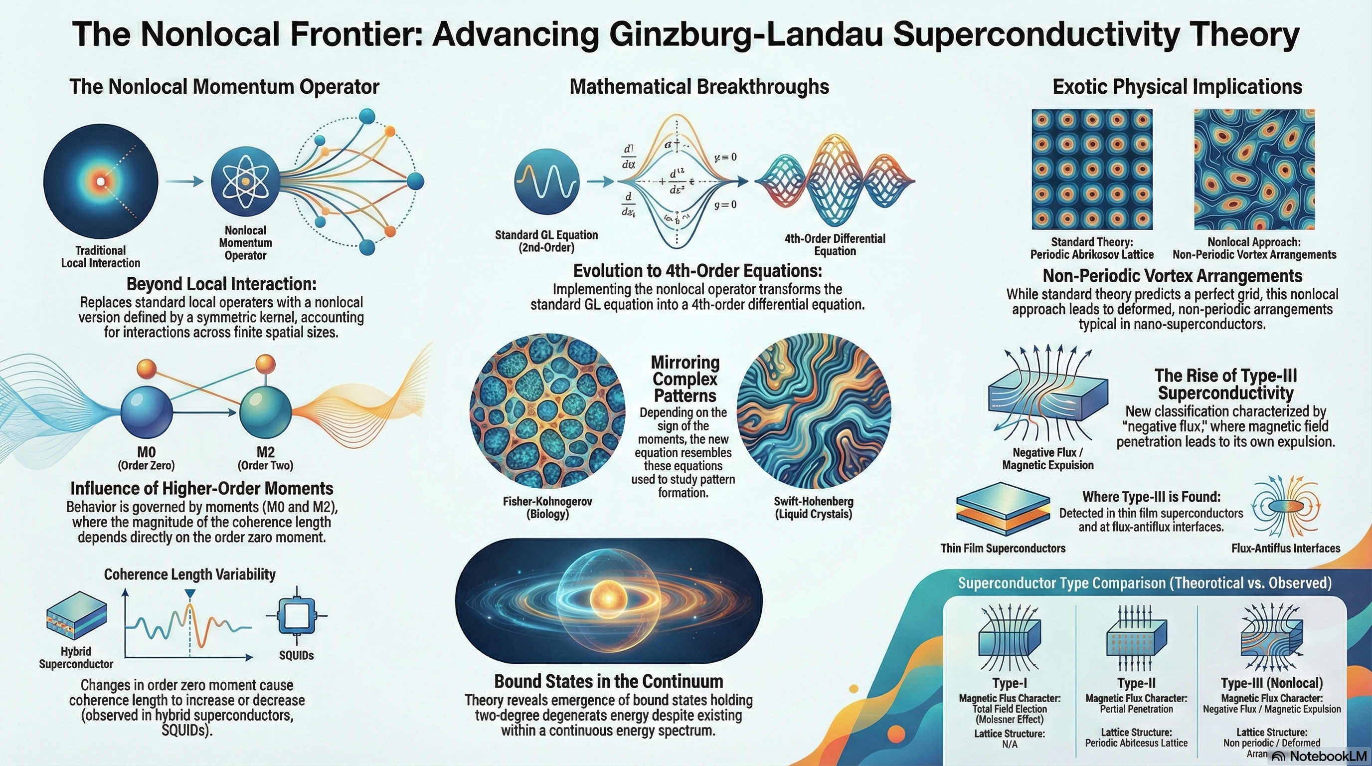
This briefing document synthesizes the findings of a 2022 study by Rami Ahmad El-Nabulsi and Waranont Anukool regarding the extension of Ginzburg-Landau (GL) superconductivity through a nonlocal momentum operator. By incorporating higher-order moments and a symmetric kernel, the researchers derived a higher-derivative superconductivity theory that offers new insights into macroscopic properties, vortex arrangements, and flux behavior.
Critical Takeaways:
● Nonlocal Momentum Framework: The theory utilizes an extended momentum operator ( $p̂_{NL}$ ) motivated by quantum stochastic processes, leading to 4th-order differential GL equations.
● Variable Coherence Length: The effective coherence length ( $\xi$ ) is found to be dependent on the zero-order moment ( $M_0$ ), allowing for both increases and decreases in magnitude, a phenomenon observed in semiconductors, SQUIDs, and hybrid superconductors.
● Mathematical Analogies: The derived equations correspond to the extended 4th-order Fisher-Kolmogorov equation or the Swift-Hohenberg equation, depending on the sign of the second-order moment ( $M_2$ ).
● Non-periodic Vortex Arrangements: Unlike the traditional periodic lattices predicted by Abrikosov, this nonlocal approach identifies non-periodic vortex arrangements and bound states in the continuum with two-degree degenerate energy.
● Emergence of Type-III Superconductivity: The study predicts the existence of Type-III superconductors characterized by negative magnetic flux, a property detected in thin films and flux-antiflux interfaces.
1. Theoretical Foundation: The Nonlocal Momentum Operator
The research shifts away from traditional local descriptions of superconductivity to address nonlocality, which is inherently linked to the finite spatial size of Cooper pairs.
1.1 The Operator Construction
The core innovation is the definition of the nonlocal momentum operator ( $p̂_{NL}$ ):
● Kernel Integration: It employs a symmetric kernel function $K(r – r’)$ where nonlocal interactions are taken into account.
● Moment Components: The operator is characterized by even moments ( $M_0, M_2, …$ ), where $M_{2m} = \frac{1}{(2m)!} \int R^{2m} K(R) dR$ .
● Expansion: For practical analysis, the operator is reduced to: $$p̂_{NL} = -i\hbar M_0\nabla – i\hbar M_2\nabla^3 – O(\hbar M_4)$$
1.2 Modified Ginzburg-Landau Equations
Implementing this operator into the GL functional leads to higher-order Euler-Lagrange equations. In the absence of an external magnetic field, the simplified nonlocal GL equation for the pseudo-wavefunction ( $\Psi$ ) is: $$\tilde{\alpha}\Psi + \tilde{\beta}|\Psi|^2\Psi – \frac{\hbar^2 M_0^2}{4m}\Delta\Psi – \frac{\hbar^2 M_0 M_2}{2m}\Delta^2\Psi = 0$$
2. Macroscopic Properties and Mathematical Solutions
The introduction of higher-order derivatives changes the fundamental mathematical nature of the GL equations, aligning them with established patterns in other fields of physics.
2.1 Mathematical Classifications
The study identifies that the behavior of the superconducting material is governed by the sign of the second-order moment $M_2$ :
● Negative $M_2$ : The equation is comparable to the extended 4th-order Fisher-Kolmogorov time-independent equation, used in pattern formation for bi-stable systems and liquid crystals.
● Positive $M_2$ : The equation resembles the Swift-Hohenberg equation, fundamental to spatiotemporal pattern formation in extended systems.
2.2 Effective Coherence Length ( $\xi$ )
The coherence length, which characterizes the scale of the superconducting electron density variations, is modified by the zero-order moment ( $M_0$ ):
● Scaling: $\xi^2_{effective} = -\frac{\hbar^2 \sigma^2}{4m\tilde{\alpha}}$ (where $\sigma$ represents $M_0$ ).
● Decrease ( $\sigma < 1$ ): Detected in commercial YBCO tapes, micro-SQUIDs, and hybrid superconductors.
● Increase ( $\sigma > 1$ ): Observed in nanomaterials like NbN films (where thickness reduction affects $T_c$ ) and multiband iron-based superconductors (e.g., LiFeAs).
3. Nonlocal Superconductivity in Bulk and Vortex Theory
The research extends Abrikosov’s theory of periodic vortex lattices to accommodate the complexities introduced by nonlocality.
3.1 Bound States in the Continuum (BSC)
A significant finding is the emergence of bound states in the continuum. In quantum mechanics, these are unusual states where wavefunctions are spatially bounded despite having continuous energies. In this theory, these states hold a two-degree degenerate energy , indicating that stable bound wavefunctions can exist under the influence of nonlocality.
3.2 Deformation of the Abrikosov Lattice
While Abrikosov’s original theory predicts regular, periodic arrays of vortices (typically hexagonal), the nonlocal framework reveals:
● Non-periodic Arrangements: Nonlocality causes a deformation of the vortex lattice, leading to periodically indistinct lattices or quasi-periodic structures.
● Practical Occurrences: This deformation is expected in superconducting nanosystems, non-periodic pinning arrays, and lattices surrounded by relaxing vortices.
4. Anomalous Flux and Type-III Superconductivity
The study highlights the emergence of “Type-III” behavior, expanding the classification beyond the traditional Type-I (complete Meissner effect) and Type-II (vortex state).
4.1 Negative Magnetic Flux
The analysis predicts a transition into a state characterized by negative magnetic flux ( $\Phi_0 < 0$ ).
● Mechanism: Negative flux penetration leads to the expulsion of the magnetic field through nonlinear screening.
● Barriers: This phenomenon is linked to high physical barriers at the superconducting boundary, such as Bean–Livingston barriers, which prevent standard quantized penetration.
4.2 Comparison of Superconductor Types
Feature,Type-I,Type-II,Type-III (Nonlocal)
Meissner Effect,Complete,Partial (in mixed state),Modified (expulsion via negative flux)
Critical Fields,Single $H_c$,$H_{c1}$ and $H_{c2}$,”$H_{c1}, H_{c2},$ and $H_{c3}$”
Vortex Structure,None,Periodic (Abrikosov),Non-periodic / Deformed
Flux Sign,Positive,Positive,Negative (Flux-Antiflux)
4.3 Detection and Observations
Negative flux and flux-antiflux interfaces are not merely theoretical; they have been detected in:
● High-temperature ( $T_c$ ) superconducting films.
● Thin films and superlattices.
● Superconductors exhibiting negative magnetoresistance.
5. Conclusion
The utilization of a nonlocal momentum operator provides a robust platform for engineering exotic superconducting phenomena. By accounting for higher-order moments, the theory successfully explains variations in coherence length, the existence of bound states in the continuum, and the non-periodic nature of vortices in nanomaterials. Furthermore, the prediction of Type-III superconductivity and negative flux offers a new direction for exploring the electromagnetic properties of thin films and hybrid superconducting systems.
Executive Summary
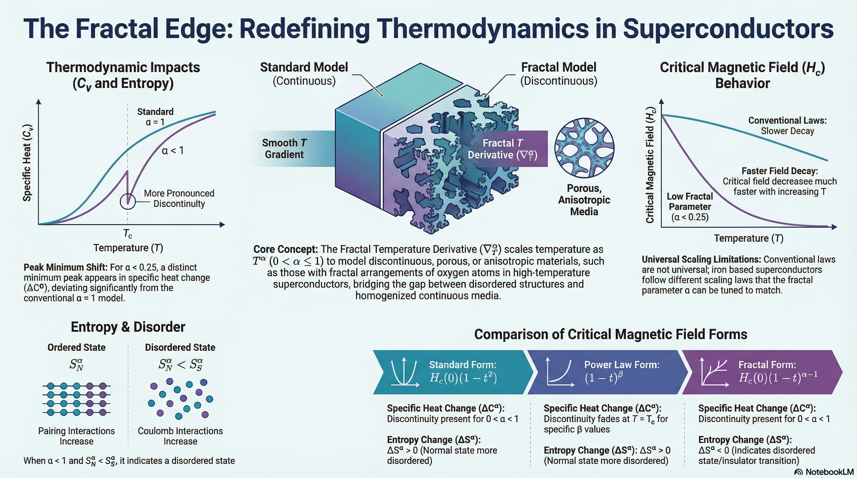
This document synthesizes findings from research exploring the application of fractal thermodynamics to superconducting phase transitions. By introducing the “fractal temperature derivative,” researchers have developed a theoretical framework to analyze the thermodynamic properties—specifically entropy, specific heat, and critical magnetic fields—of anisotropic and disordered superconductors.
Critical Takeaways:
● Fractal Temperature Derivative: Utilizing the Li and Ostoja-Starzewski (LOSA) approach, the research models temperature as a fractal measure, allowing for the analysis of discontinuous fractal media where conventional calculus fails.
● Enhanced Modeling of Disorder: The fractal approach is particularly effective for modeling “strongly disordered” superconductors and high-temperature superconductors, which possess internal fractal structures related to oxygen atom arrangements and porous geometries.
● Thermodynamic Anomalies: The study reveals that the fractal parameter ( $\alpha$ ) significantly influences the behavior of specific heat and the decay rate of the critical magnetic field. Specifically, for $\alpha < 1$ , the model predicts discontinuities and ordering effects that align with experimental observations in materials like iron-based superconductors and heavy-fermion paramagnets.
● Phase Transition Insights: The research demonstrates that the superconducting state in these fractal systems is more ordered than the normal state, with the entropy of the normal state consistently exceeding that of the superconducting state under standard conditions.
1. Conceptual Framework: Fractal Temperature in Superconductors
Traditional thermodynamics assumes a continuous space, which often fails to accurately represent the behavior of porous and anisotropic media. Superconductors often possess internal fractal structures that are essential for high-temperature functionality and efficient heat dissipation via refrigerant diffusion through pores.
1.1 The Fractal Derivative Approach
The research adopts the “fractal temperature derivative” (LOSA approach), defined as: $$\nabla_T^\alpha := \left(\frac{T_0}{T_c – T}\right)^{\alpha-1} \nabla T$$ where:
● $\alpha$ : The fractal parameter ( $0 < \alpha \le 1$ ).
● $T_c$ : The critical temperature.
● $T_0$ : The initial heater temperature, typically close to $T_c$ .This local operator bridges discontinuous fractal media with homogenized continuous media, providing a more practical tool for materials like $MgB_2$ (magnesium diboride), which exhibit significant anisotropy.
1.2 Thermodynamic Reversibility
Because the transition between normal and superconducting states is thermodynamically reversible (the Meissner effect), thermodynamics can be applied to the phase transition. The fractal derivative is used to redefine the entropy ( $S_\alpha$ ) and specific heat ( $C_\alpha$ ) based on the gradient of the Gibbs free energy ( $G$ ) in fractal media.
2. Impact on the Paramagnetic Meissner Effect
The study examines the paramagnetic Meissner effect in small anisotropic superconductors, focusing on how fractal temperature influence the transition between the normal ( $N$ ) and superconducting ( $S$ ) states.
2.1 Entropy and Order
The difference in fractal entropy ( $\Delta_\alpha S$ ) between the two states indicates that for $T < T_c$ , the superconducting state is more ordered than the normal state ( $S_\alpha^N > S_\alpha^S$ ).
● In disordered states, increased Coulomb interactions can decrease pairing interactions, potentially leading to a transition from a superconducting state to an insulating state.
● High-critical temperature superconductors are fundamentally characterized as disordered.
2.2 Fractal Specific Heat ( $C_\alpha$ )
The heat capacity of a material—representing the thermal energy required to increase temperature—is highly sensitive to phase changes. The fractal model reveals:
● Discontinuity: For $\alpha < 1$ , a discontinuity in specific heat occurs during the temperature transition.
● Peak Variations: Numerical analysis shows that for $\alpha < 0.25$ , a minimum peak appears for $\Delta C_\alpha$ (the difference between normal and superconducting specific heat).
● Extra-ordering: At very low temperatures ( $T \rightarrow 0$ ), the superconducting state rejects less heat than the normal state, leading to “extra-ordering.”
3. Critical Magnetic Field ( $H_c$ ) Dynamics
The fractal parameter $\alpha$ significantly alters the decay and behavior of the critical magnetic field ( $H_c$ ), which is the maximum field strength a superconductor can withstand while maintaining superconductivity.
● Decay Rates: As temperature increases, $H_c$ decreases. For values of $\alpha < 0.25$ , the decay of the magnetic field is slower than the conventional decay (which occurs at $\alpha = 1$ ).
● Scaling Laws: The research introduces various analytical forms of the critical magnetic field to match experimental observations in different materials, such as $Nb_3Ge$ films and $Ba-122$ single crystals.
● Non-monotonicity: Certain models describe a non-monotonic dependence of the critical current on the magnetic field, where the superconducting temperature decreases as the field increases.
4. Thermodynamical Analysis and the Order Parameter
The research utilizes Jumarie’s modified Riemann-Liouville fractional integral to analyze the Gibbs free energy in the absence of a magnetic field.
4.1 The Order Parameter ( $\omega$ )
The fraction of normal-electrons is defined by the order parameter $\omega$ .
● $\omega = n_n / N$ (Normal-electron fraction).
● $1 – \omega = n_s / N$ (Superelectron fraction).
● At equilibrium, the order parameter $\omega$ decreases rapidly with temperature, particularly when $\alpha < 0.25$ .
4.2 Low-Temperature Superconductors
For low-temperature superconductors (e.g., lead and mercury), the fractal model provides specific heat anomaly patterns that reproduce experimental data qualitatively. This is useful for studying “unconventional superconductivity” in heavy-fermion paramagnets like $UTe_2$ .
Table 1: Summary of Basic Properties for Various $H_c(T)$ Models| Property | $H_c(T) = H_c(0)(1 – t^2)$ | $H_c(T) = H_c(0)(1 – t)^\beta$ | $H_c(T) = H_c(0)(1 – t)^{\alpha-1}$ || —— | —— | —— | —— || Specific Heat ( $\Delta C_\alpha$ ) | Presence of discontinuity for $0 < \alpha < 1$ . | Absence of discontinuity at $T = T_c$ for $1/2 < \beta < 1$ . | Presence of discontinuity for $0 < \alpha < 1$ . || Entropy ( $\Delta_\alpha S$ ) | $\Delta_\alpha S > 0$ ; Normal state is more disordered. | $\Delta_\alpha S > 0$ for $T \ll T_c$ . | $\Delta_\alpha S < 0$ for $0 < \alpha < 1$ ; Presence of disorder. || State Comparison | $C_\alpha^N < C_\alpha^S$ | $C_\alpha^N > C_\alpha^S$ | $C_\alpha^N < C_\alpha^S$ |
5. Conclusions and Future Directions
The integration of fractal calculus into superconductivity theory offers a novel methodology for understanding phase transitions that cannot be captured by conventional formalisms.
● Universal Application: The fractal thermodynamical formulation can be applied to iron-based superconductors, thin films, and highly porous polycrystalline materials.
● Disorder Management: The model successfully addresses the effects of disorder on electrical resistance and the transition to insulating states.
● Future Research: Potential exists to apply this framework to superconducting anti-perovskites and bulk semiconductors. Further exploration of “two-scale fractal derivatives” may provide additional insights into fractal thermodynamics and its correlation with electronic properties.
Executive Summary
The Metal Oxide Semiconductor Field Effect Transistor (MOSFET) is a foundational component of modern computer engineering and nanotechnology. As device scaling reaches the nanoscale, classical physics becomes insufficient for predicting performance, necessitating a transition to quantum mechanical models. This research investigates the quantum effects in MOSFETs through the lens of fractal dimensions, specifically utilizing the Product-Like Fractal Measure (PLFM) to model anisotropic nanostructures.The analysis demonstrates that fractal patterns emerge naturally in self-assembled metallic nanoparticles and electronic circuits. By applying the Li and Ostoja-Starzewski approach (LOSA) to the Poisson and Schrödinger equations, the study determines that the fractal dimension ( $\alpha$ ) for these devices is approximately 0.66 , falling within the critical range of $1/2 < \alpha < 2/3$ . These findings provide a more accurate assessment of carrier density reallocation near the $Si-SiO_2$ interface, offering a vital framework for the development of ultra-thin, highly doped nanoelectronic devices.
The Role of Fractals in Nanoelectronics
Traditional semiconductor modeling often assumes homogeneity, yet real-world nanofilms (such as single-layer graphene or Bi films) exhibit quasi-discrete features in their energy spectrum. In nano-devices like MOSFETs, self-assembly processes frequently generate fractal patterns where millions of metallic nanoparticles form complex, self-similar circuits.
Limitations of Classical Physics
At the nanoscale, classical predictions of carrier behavior fail. Quantum mechanical effects cause a significant reallocation of carrier density close to the Silicon-Silicon Dioxide ( $Si-SiO_2$ ) interface. Understanding these effects is critical for:
● Assessing the scaling limits of MOSFETs.
● Designing Complementary Metal-Oxide-Semiconductor (CMOS) digital circuits.
● Modeling low-frequency $1/f$ noise and soft breakdown in ultra-thin transistors.
MOSFET Structure and Operational Principles
The MOSFET is a three-terminal microelectronic device composed of a Gate (G), Source (S), and Drain (D). It operates primarily as a digital switch for controlling loads in computer architectures.
Device Architecture
As illustrated in the provided source context, the physical structure consists of:
● Gate Oxide ( $SiO_2$ ): A very thin dielectric layer separating the gate terminal from the conductive channel.
● Channel Region: The area between the source and drain where the transistor “turns on.”
● Substrate (Body): A P-type substrate in standard configurations.
● Depletion Layer: A region formed under the gate oxide where mobile charge carriers are depleted.
Switching Mechanisms
The operational behavior depends on the channel type:| MOSFET Type | Activation Condition | Operation Region || —— | —— | —— || N-Channel | Gate voltage relative to Source exceeds a positive threshold. | Operates between cut-off and saturation. || P-Channel | Gate voltage relative to Source is negative. | Operates between cut-off and saturation. |
Theoretical Framework: Product-Like Fractal Measure (PLFM)
To describe anisotropic devices, the study adopts the Li and Ostoja-Starzewski approach (LOSA) . This framework is particularly suited for inhomogeneous nanostructures where mass and density are distributed across fractal dimensions ( $\alpha_k$ ).
Key Mathematical Operators
The LOSA approach introduces specialized operators to handle fractal geometry:
● Fractal Gradient Operator ( $\nabla_D$ ): Utilizes a volume transformation coefficient to account for the fractal nature of the medium.
● Fractal Laplacian Operator ( $\Delta_\alpha$ ): Emerges from the application of the Gauss theorem to fractal surfaces.
● Potential Distribution: Described by a fractal version of the Poisson equation, accounting for depletion charge density ( $N_A$ ) and inversion charge density ( $n$ ).
Quantum Confinement and Subband Modeling
Quantum confinement occurs when particles are restricted by a potential barrier, leading to discretized energy levels. In MOSFETs, this is most significant in the direction normal to the gate due to the strong electric field.
Fractal Schrödinger Equation
The study employs a fractal version of the Schrödinger equation to determine energy levels ( $E_i$ ) and carrier wavefunctions ( $\psi_i$ ). Because the lowest two subbands account for 80–95% of the total carrier population when gate voltage varies from 0 to 3 Volts, the model focuses on these primary energy levels.
Variational Method Results
The analysis identifies two sets of masses for silicon interfaces parallel to the 100 plane:
Longitudinal Mass ( $m_1$ ): $0.916m_0$ along the $<100>$ axis.
Transverse Mass ( $m_2$ ): $0.19m_0$ .By applying the variational method to minimize energy, the research derives parameters for the electron density peaks in different “valleys” of the semiconductor structure.
Findings and Numerical Estimates
The research provides specific insights into the behavior of the potential and wavefunctions within fractal dimensions.
Potential and Wavefunction Variations
● Potential ( $\phi_{dep}$ ): For low fractal dimensions (e.g., $\alpha = 0.25$ ), there is a large increase in potential. As the fractal dimension approaches unity (integer dimension), the variation becomes smaller.
● Wavefunction ( $\psi_{11}$ ): The wavefunction is bounded specifically when the fractal dimension lies between $1/2$ and $2/3$ . Outside this range, the wavefunction tends to increase, which may not align with physical constraints in a confined system.
Estimation of the Fractal Dimension
By comparing the theoretical model with observations of inversion charges at high operating bias, the study concludes:
● The parameter $\xi$ (related to effective masses) is approximately 0.6.
● The estimated fractal dimension for the MOSFET system is $\alpha \approx 0.66$ .
Conclusion and Future Implications
The integration of fractal calculus into quantum mechanical MOSFET modeling offers a robust alternative to classical physics at the nanoscale. By identifying the fractal dimension as approximately 0.66, researchers can better predict the reallocation of carriers at the $Si-SiO_2$ interface.This methodology extends beyond silicon transistors and may be applied to:
● Supercapacitors: Modeling electrostatics in activated-carbon electrodes.
● Optoelectronics: Analyzing semiconductor alloys and organic thin films.
● Disordered Materials: Investigating highly disordered or inhomogeneous systems where classical Euclidean geometry fails to capture the underlying physics.
Executive Summary
Research published in February 2026 identifies a direct correlation between field-theoretic modifications of the electromagnetic Lagrangian and the quantum entanglement properties of photonic systems. By introducing a small deformation parameter ( $\epsilon$ ) to the standard Maxwellian Lagrangian ( $L \rightarrow aL^{1+\epsilon}$ ), the study demonstrates that even infinitesimal nonlinearities influence photon correlations, coherence, and von Neumann entropy.
Critical takeaways include:
● Universal Entropy Reduction: For maximally entangled two-photon and GHZ states, Lagrangian deformations cause a universal quadratic reduction in entropy ( $S \approx \ln 2 – \delta^2/2$ ). This confirms that maximal entanglement represents a local maximum of entropy.
● State-Dependent Sensitivity: Multi-photon entangled states exhibit distinct scaling behaviors. GHZ states are characterized by “fragility,” showing quadratic scaling of entropy reduction relative to subsystem size. Conversely, W-type states demonstrate “robustness” with linear scaling, as entanglement is shared more redundantly across the system.
● Frequency Dependence: The deformation introduces a mode-dependent scaling of field operators. Consequently, entanglement entropy inherits a dependence on photon frequency, suggesting that high-frequency photons are more sensitive probes for detecting deviations from Maxwellian linearity.
● Entanglement Rebalancing: While deformations typically reduce entanglement in maximally entangled states, they can enhance entanglement in non-maximally entangled pure states by redistributing probability amplitudes toward equal Schmidt weights.
1. Theoretical Framework: Deforming the Electromagnetic Lagrangian
The investigation centers on the transition from conventional linear quantum electrodynamics (QED) to a modified theory. In standard QED, the Lagrangian is quadratic in the field strength tensor, ensuring the linear propagation of photons.
1.1 The Modified Lagrangian
The study utilizes a generalized power-law expression: $$L_{mod} = aL^{1+\epsilon} = aL(1 + \epsilon \ln L) + O(\epsilon^2)$$ Where:
● $a$ : A coupling constant related to a mass scale.
● $\epsilon$ : A small deformation parameter quantifying deviations from standard quadratic scaling.
● $L_{int} = a\epsilon L \ln L$ : The resulting weak nonlinear interaction term.This modification introduces effective photon-photon vertices (3- and 4-photon couplings) similar to Euler-Heisenberg or Born-Infeld models. These vertices modify free propagators and produce vacuum polarization effects.
1.2 Field-Theoretic Corrections
To evaluate entanglement accurately, the study utilizes corrected two-point functions that encode propagation and correlations.
● Loop Integrals: Interactions manifest through loop integrals analogous to photon-photon scattering.
● Connected Diagrams: Only connected diagrams contribute to genuine correlations between subsystems. Disconnected diagrams factorize and do not influence entanglement measures like von Neumann entropy.
● Time-Evolution: The time-evolution operator $U_I(t, t_0)$ is expanded to first order in $\epsilon$ to compute S-matrix elements for small finite Hilbert spaces (e.g., two-photon or cavity modes).
2. Impact on Two-Photon Polarization Entanglement
Using states generated via spontaneous parametric down-conversion (SPDC), the analysis examines how deformations modify the reduced density matrices of entangled photons.
2.1 Mode-Dependent Scaling
The deformation $L \rightarrow aL^{1+\epsilon}$ rescales photon creation and annihilation operators. For a vector potential $A_i$ , the factor $L^\epsilon$ introduces a mode-dependent scaling: $$a^\dagger_{k,\lambda} \rightarrow (1 + \epsilon \langle \ln L \rangle) a^\dagger_{k,\lambda}$$ This scaling produces a slight imbalance in superposition amplitudes, causing a maximally entangled Bell state to become slightly non-maximal.
2.2 Entropy Correction for Two-Photon States
For a maximally entangled Bell-like state, the von Neumann entropy ( $S$ ) following deformation is: $$S \approx \ln 2 – \frac{1}{2} \delta^2 + O(\delta^3)$$ Where $\delta = \epsilon \langle \ln L \rangle$ .
● Symmetry: The leading correction is quadratic because entropy is maximal at $\delta = 0$ .
● Frequency Sensitivity: Taking $\ln L \approx \ln \omega$ , the correction for visible photons ( $\omega \approx 10^{15}$ Hz) suggests that even minute values of $\epsilon$ produce a measurable reduction in entanglement.
3. Multi-Photon Entanglement: GHZ vs. W-States
The study extends the analysis to $N$ -photon systems, revealing that the internal structure of entanglement dictates the system’s resilience to Lagrangian deformations.
3.1 GHZ States: Fragility
Greenberger-Horne-Zeilinger (GHZ) states represent maximal entanglement across $N$ photons.
● Scaling: The entropy reduction scales quadratically with the number of photons traced out ( $k^2$ ).
● Sensitivity: Because GHZ entanglement is concentrated in a single global coherence between two distinct components, any perturbation leads to rapid degradation.
● Entropy Result: $S_k \approx \ln 2 – \frac{k^2 \delta^2}{2}$ .
3.2 W-States: Robustness
$N$ -photon W-states retain partial entanglement even if photons are lost.
● Scaling: These states exhibit linear scaling of entropy reduction.
● Mechanism: Entanglement in W-states is shared redundantly among many photons. Small, distributed changes across many orthogonal components result in a parametrically smaller total entropy loss compared to GHZ states for a given subsystem size.
● Entropy Result: $S_k(1) \approx S_k(0) – \frac{1}{2} \sum_{i=1}^k (\epsilon \log_2 \omega_i)^2$ .
Comparison of Entanglement Systems
System,Entanglement Type,Leading-Order Entropy Effect,Characterization
Two-Photon,Polarization,$S \approx \ln 2 – \delta^2/2$,Universal Quadratic Reduction
GHZ State,Multi-photon,$S_k \approx \ln 2 – k^2\delta^2/2$,Fragile / Highly Sensitive
W-State,Multi-photon,$S_k \approx S_k(0) – \text{linear terms}$,Robust / Distributed
4. General Principles of Entanglement Rebalancing
A critical finding is that Lagrangian deformation does not universally destroy entanglement. Instead, it acts as a “rebalancing mechanism” for Schmidt coefficients.
4.1 Enhancement of Non-Maximal States
For pure bipartite states that are not initially maximally entangled, the deformation can push probabilities toward equality.
● Linear Change: If the initial state is non-maximal, the entropy change is linear in $\delta$ . The sign of the change depends on whether the deformation pushes the Schmidt weights toward or away from $1/2$ .
● Theorem of Impossibility: If the initial state is already maximally entangled within its support, enhancement is impossible; the linear term vanishes, and the leading correction is always negative and quadratic.
4.2 Frequency-Dependent Renormalization
Frequency enters the calculation through a mode-dependent wave-function renormalization factor $Z(\omega) = 1 + \epsilon g(\omega)$ .
● Amplitudes: Deformations rescale amplitudes in a frequency-dependent way ( $c_j \rightarrow c_j \sqrt{Z(\omega_j)}$ ).
● Transfer Function: The function $g(\omega)$ acts as a transfer function, converting microscopic Lagrangian deformations into macroscopic, frequency-dependent modifications of entanglement.
5. Conclusion and Experimental Implications
The study establishes that precision measurements of entanglement in photonic systems can serve as sensitive probes for weak nonlinearities in electromagnetic dynamics.
High-Energy Probing: The logarithmic dependence on frequency ( $\ln \omega$ ) implies that high-energy photons are the most effective tools for detecting infinitesimal field-theoretic deformations.
Structural Integrity: The choice of entangled state (GHZ vs. W) is paramount when designing experiments to test Lagrangian stability, as W-states will maintain their entanglement profile longer under perturbative stress.
Physical Consistency: The analysis confirms that normalization in multi-photon states arises from sums of squared amplitudes rather than products, ensuring consistency in entropy calculations across complex photonic architectures.
http://rcqt.science.cmu.ac.th/wp-content/uploads/2026/13Casimir effect associated – Eng.png
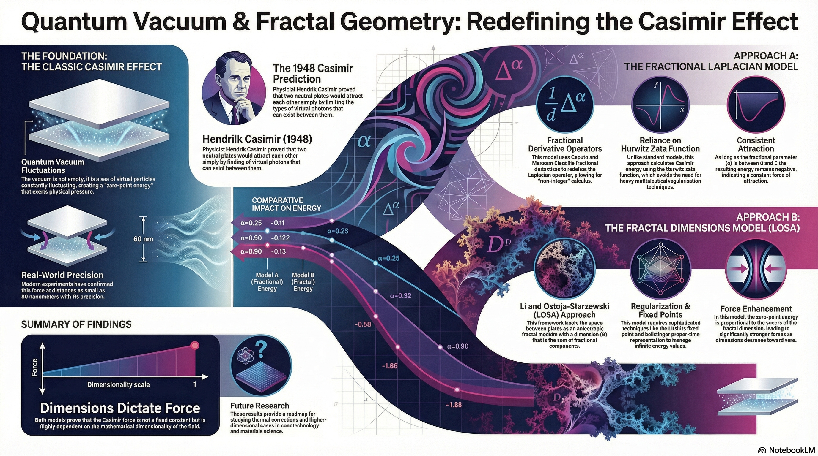
Executive Summary
This briefing document synthesizes research published in Physica E regarding the mathematical and physical re-evaluation of the Casimir effect through the lenses of fractional calculus and fractal geometry. The Casimir effect—traditionally the attractive force between two neutral parallel plates caused by quantum vacuum fluctuations—is shown to be significantly modified when space is modeled using fractional or fractal dimensions.
Two distinct methodologies are explored:
Fractional Laplacian Approach: Utilizing Caputo and Riemann-Liouville fractional derivatives, this model calculates Casimir energy via the Hurwitz zeta function, finding that energy is negative (attractive) for fractional orders between zero and one.
Fractal Dimension Approach (LOSA): Applying the Li and Ostoja-Starzewski approach to anisotropic media, this model demonstrates that zero-point energy depends on the square of the fractal dimension. Crucially, the Casimir force is significantly enhanced at lower fractal dimensions.The study concludes that vacuum energy and its resulting pressure are fundamentally dependent on the fractional order parameters and the numerical values of fractal dimensions, providing new insights into quantum field theory applications from nanoscales to large-scale physics.
1. Introduction to the Casimir Effect
The Casimir effect, first predicted by Hendrik Brugt Gerhard Casimir in 1948, describes the small attractive force between a pair of neutral, parallel conducting plates. This phenomenon is a cornerstone of quantum field theory, based on several key postulates:
● Quantum Vacuum Fluctuations: The vacuum is not empty but consists of virtual particles in a continuous state of fluctuation (creation and annihilation).
● Energy Deformation: The presence of conducting plates restricts the wavelengths of virtual photons that can exist between them. Only wavelengths that fit a complete number of times are counted, leading to a decrease in energy density as plates move closer.
● Resultant Force: This decrease in energy density creates a pressure change, known as the Casimir force, which draws the plates together.While traditional calculations use Dirichlet or Neumann boundary conditions and Riemann zeta function regularization, recent research has expanded these boundaries into fractional and fractal mathematics.
2. Methodology I: The Fractional Laplacian Approach
The first approach explores the Casimir effect through generalized fractional Laplace operators based on Caputo (order $\delta$ ) and Riemann-Liouville (order $\omega$ ) derivatives.
Mathematical Framework
● Fractional Operators: The model uses a generalized fractional Laplace operator defined by the combination of these derivatives.
● Schrödinger Boundary Value Problem: The solution involves the Mittag-Leffler function , a generalization of the exponential function used in fractional calculus.
● Energy Calculation: Unlike the standard approach, this model utilizes the Hurwitz zeta function ( $\zeta_H$ ) to sum possible modes and calculate the zero-point energy ( $E_0$ ).
Key Findings and Evidence
The research indicates that as long as the fractional order parameter ( $\alpha$ ) remains between 0 and 1, the energy remains negative, signifying a positive force of attraction.Energy Values for Specific Fractional Orders ( $\alpha$ ): | Fractional Order ( $\alpha$ ) | Calculated Casimir Energy ( $E_0$ ) | | :— | :— | | $\alpha = 1/4$ | $\approx -0.11$ | | $\alpha = 1/2$ | $\approx -0.122$ | | $\alpha = 0.9$ | $\approx -0.13$ |Notable Observation: In this model, the regularization technique is not “strongly required” because the Hurwitz zeta function naturally handles the summation for these specific boundary conditions.
3. Methodology II: The Fractal Dimension Approach (LOSA)
The second approach utilizes the Li and Ostoja-Starzewski Approach (LOSA) , which describes physical systems in anisotropic media with fractal dimensions ( $D = \alpha_1 + \alpha_2 + \alpha_3$ ).
Mathematical Framework
● Fractal Gradient and Laplacian: This method defines length, surface, and volume measures in terms of fractal dimensions ( $\alpha_k$ ). It relates fractal volume elements to standard Euclidean elements through transformation coefficients.
● Regularization Techniques: Unlike the first model, this approach requires sophisticated regularization:
● Lifshitz Fixed Point: Modified with a parameter $\xi$ .
● Schwinger Proper-Time Representation: Used to handle the summation of infinite modes.
Key Findings and Evidence
In this model, the zero-point energy depends on the square of the fractal dimension ( $\alpha^2$ ).Energy Values for Specific Fractal Dimensions ( $\alpha$ ) at $\xi = 1$ : | Fractal Dimension ( $\alpha$ ) | Calculated Casimir Energy ( $E_0$ ) | | :— | :— | | $\alpha = 1/4$ | $\approx -0.145$ | | $\alpha = 1/2$ | $\approx -0.58$ | | $\alpha = 0.9$ | $\approx -1.88$ |Force Enhancement: A critical takeaway from this approach is that the Casimir force is “much bigger” than the basic result obtained for a standard massless scalar field when fractal dimensions are lower (close to zero).
4. Comparative Analysis of Approaches
The research highlights distinct differences in how fractional and fractal mathematics affect the interpretation of the Casimir effect:| Feature | Fractional Laplacian Approach | Fractal Dimension (LOSA) Approach || —— | —— | —— || Primary Operator | Caputo & Riemann-Liouville Derivatives | Fractal Gradient & LOSA Laplacian || Mathematical Tool | Hurwitz Zeta Function | Lifshitz Fixed Point & Schwinger Proper-Time || Regularization | Not strongly required | Essential/Required || Energy Dependency | Affected by fractional order parameter | Depends on the square of fractal dimension || Force Impact | Slight modification of energy/pressure | Significant enhancement at lower dimensions |
5. Conclusions and Future Directions
The study successfully demonstrates that the Casimir effect is highly sensitive to the geometric and analytical structure of the space in which fields fluctuate.
Central Insights
● Mathematical Versatility: Fractional calculus provides a bridge to interpolate between different boundary conditions (Dirichlet and Neumann).
● Dimension Sensitivity: Both fractional operators and fractal dimensions fundamentally alter the zero-point energy of the vacuum.
● Nanoscale Implications: Because the Casimir effect plays a leading role in nanoscales (distances as small as 60 nm have been measured), these models are vital for precision engineering and theoretical physics.
Proposed Future Research
The authors suggest extending these findings by:
● Analyzing higher-dimensional cases.
● Studying thermal corrections to both fractional and fractal Casimir effects.
● Investigating the “massive” case (particles with mass) using dimensional regularization.
6. Significant Quotes
“The vacuum is not empty but consists of particles which are in a continuous state of fluctuations and can cause a force of attraction.””The Casimir energy and force are obtained throughout the Hurwitz zeta function and not by means of the Riemann zeta function in the fractional model.””For lower values of fractal dimensions, the force is much bigger than the basic result obtained by Casimir for a D massless scalar field.”
Executive Summary
This briefing document synthesizes research published in Chaos, Solitons and Fractals (2023) regarding the construction and analysis of three distinct forms of nonlinear Schrödinger equations (NSE). The study, authored by Rami Ahmad El-Nabulsi and Waranont Anukool, explores the nonlocal aspects of quantum theory and fractional quantum mechanics to describe systems with long-range interactions, such as energy transport in biomolecules and nonlinear optics.
The investigation utilizes three primary analytical frameworks:
Nonlocal generalized fractional momentum operators (mixed fractional Laplacians).
Fractional Riccati methods (modified Riemann–Liouville derivative operators).
Laplacian operators in fractal dimensions (the Li and Ostoja-Starzewski approach).Critical Takeaways:
● Methodological Comparison: The first two approaches yield comparable solutions, while the third approach produces an NSE with variable coefficients, facilitating a significantly larger family of solitonic solutions.
● De-fractionalization: Under specific constraints (e.g., $\alpha + \beta = 1$ ), fractional equations can be reduced to integer-order equations, such as the Fisher-Kolmogorov equation, which are widely used in quantum optics.
● Stability and Nonlocality: The presence of nonlocal kernels is identified as a critical factor in preventing collapse in the nonlocal NSE.
● Soliton Diversity: The research demonstrates the emergence of various soliton types, including “breathers,” bright solitons (localized intensity peaks), and combined bright-dark solitons, depending on the fractional parameters and scales involved.
Theoretical Foundations of Nonlocal NSE
The research is motivated by two pillars of modern theoretical physics: the nonlocal nature of quantum theory (essential for quantum information processing and entanglement) and the fractional formulation of quantum mechanics.
Core Concepts
● Nonlocal Interactions: These are characterized by convolutions with kernels that analyze the behavior of dynamical systems in biology, chemical physics, and reaction-diffusion systems.
● Fractional Quantum Mechanics: This field describes hidden properties of systems with long-range interactions, such as charge storage in biomolecules.
● Solitons: These are defined as nonlinear localized bound states—very narrow optical pulses—that maintain their shape despite dispersion and nonlinearities.
Analysis of the Three Analytical Approaches
Approach A: Nonlocal Generalized Fractional Momentum Operator
This method derives the NSE from an operator characterized by mixed fractional Laplacians of various orders.
● Mathematical Framework: The square of the momentum operator is defined using symmetric kernels $K(x-x’)$ . This generalizes the fractional Laplacian operator found in existing literature.
● Key Findings:
● Mixed Orders: The resulting equation belongs to a class of NSE characterized by mixed fractional Laplacian orders.
● De-fractionalization: When $\alpha = \beta = 1$ , the equation reduces to a 4th-order quantum derivative equation, also known as the Fisher-Kolmogorov equation.
● Soliton Stability: Numerical analysis indicates that solutions are stable for $1/2 < \alpha + \beta \leq 1$ .
● Solitonic Behavior: For $\alpha + \beta = 1$ , the study identifies a stable “breather” soliton. At large space and time scales, these appear as “bright solitons”—localized intensity peaks above a continuous wave background that propagate periodically.
Approach B: Fractional Riccati Method
This approach introduces a space-time fractional NSE using modified Riemann-Liouville derivative operators.
● Mathematical Framework: This method relies on the Mittag-Leffler type function and symmetric kernels to simplify the momentum operator.
● Key Findings:
● Temporal Dominance: For the constraint $\beta = 1 – \alpha$ , the spatial component de-fractionalizes, resulting in an equation that is fractional only in time while maintaining an integer-order Laplacian.
● Analytical Solutions: Solutions are obtained via the Sumudu decomposition method, particularly for cases involving negative potentials (e.g., $W(x) = -\cos^2x$ ).
● Solitonic Behavior: The solitons obtained here exhibit “strange structures” and periodic dynamics. The dynamics based on modified Riemann-Liouville operators differ significantly from those based on fractional Laplacians.
Approach C: Laplacian Operator in Fractal Dimensions
This method utilizes the Laplacian operator for fractal dimensions ( $0 < \alpha \leq 1$ ) within the framework of “product-like fractal measure” for anisotropic continuum media (the LOSA approach).
● Mathematical Framework: This approach uses transformation coefficients ( $c_1, c_2, c_3$ ) to connect fractal line, surface, and volume elements to their Euclidean counterparts. It introduces a fractal gradient operator.
● Key Findings:
● Variable Coefficients: This approach is unique because it results in an NSE with variable coefficients.
● Equation Reduction: For suitable fractional parameters, the equation can be reduced to a nonlinear partial differential equation comparable to the standard NSE.
● Solitonic Behavior:
● Small Scales: Describes single solitons and combined bright-dark solitons.
● Large Scales: Describes multi-soliton interactions and waves with different wavelengths.
Comparative Summary of Methods
Feature,Mixed Fractional Laplacians (A),Fractional Riccati Method (B),Fractal Dimensions/LOSA (C)
Operator Basis,Mixed fractional Laplacians,Riemann-Liouville derivatives,Fractal gradient/Laplacian
Coefficient Type,Constant coefficients,Constant/Fractional parameters,Variable coefficients
Primary Soliton Type,Breathers / Bright solitons,”Periodic / “”Strange”” structures”,Single & Multi-soliton interactions
Complexity,High (Mixed orders),Moderate (Standard fractional),Highest (Anisotropic/Variable)
Stability,Proved for $1/2 < \alpha + \beta \leq 1$,Dependent on approximate order,Highly dependent on scale
Physical Implications and Applications
The family of NSEs constructed in this study offers broad applicability across several domains of physics and engineering:
● Nonlinear Optics: Analysis of optical solitary waves, the Kerr effect, and propagation in monomode dielectric waveguides.
● Quantum Fluids: Insights into Bose-Einstein condensation and superfluid Bose-Fermi mixtures.
● Plasma Physics: Modeling hydro-magnetic waves in cold plasma and electron acoustic solitons in unmagnetized plasma.
● Nuclear Engineering: Implications for fractal neutron transport and fuel burn-up in nuclear reactors.
● Biological Systems: Modeling energy and charge transport in complex biomolecules and biomembranes.
Conclusion
The study successfully demonstrates that a generalized fractional NSE can be constructed using a kernel approach. While many fractional nonlinear evolution equations are non-integrable, the frameworks provided—particularly the fractal dimension approach—open new avenues for finding exact solutions to complex nonlinear phenomena. The authors conclude that the behavior of solitons is highly sensitive to the specific fractional or fractal methodology employed, with nonlocal kernels serving as a vital stabilizing force against system collapse.
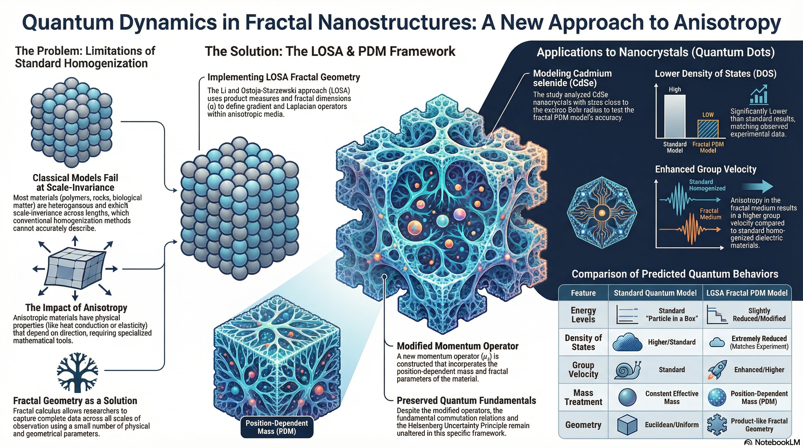
Executive Summary
The research synthesized in this document explores a novel quantum mechanical framework that integrates Li and Ostoja-Starzewski Approach (LOSA) fractal geometry with Position-Dependent Mass (PDM) . By applying this framework to low-dimensional systems, specifically semiconductor nanocrystals, the study identifies significant deviations from standard quantum mechanical models.
Key Takeaways:
● Modified Framework: The study successfully derives a modified Schrödinger equation and a generalized momentum operator ( $p̂_f$ ) that incorporates fractal anisotropy and spatial mass variation.
● Physical Consistency: Despite the modification of the momentum operator, the fundamental commutation relations and the Heisenberg uncertainty principle remain unaltered under specific parameter constraints.
● Energy Level Shifts: The energy eigenvalues for various effective potentials (inverse square root, harmonic oscillator-like) are found to be strongly influenced by the fractal parameter $\alpha$ , generally resulting in reduced energy levels compared to standard approaches.
● Nanoscale Implications: Applied to Cadmium selenide (CdSe) nanocrystals, the model predicts a density of states significantly lower than standard results and an enhanced group velocity, both of which align with observed behaviors in anisotropic homogenized dielectric media.
1. Theoretical Framework: LOSA and Fractal Geometry
The foundation of this research lies in the Li and Ostoja-Starzewski Approach (LOSA), which is designed to model physical properties in porous and anisotropic media using product-like fractal geometry.
1.1 Fractal Mass Distribution and Operators
In LOSA, mass distribution along a parallelepiped is represented through a product measure. The dimensions are defined by $D = \alpha_1 + \alpha_2 + \alpha_3$ , where $0 < \alpha_k \leq 1$ serves as the fractal dimension in the $k$ -direction.| Operator | Mathematical Representation in LOSA || —— | —— || Fractal Gradient | $\nabla_D = e_k(c_{(k)1})^{-1}\nabla_k$ || Fractal Laplacian | $\Delta_{D1} = (c_{(1)1})^{-1} \nabla ((c_{(1)1})^{-1} \nabla)$ || Length Coefficient | $c_{(k)1}(x) = l_{a,k}(x_k – x_{a,k})^{\alpha_k-1} + l_{b,k}(x_{b,k} – x_k)^{\alpha_k-1}$ |
1.2 Integration of Position-Dependent Mass (PDM)
PDM is a critical concept in solid-state physics, particularly for crystalline microstructures, semiconductors, and quantum dots. The study extends the PDM approach onto a fractal support to analyze particle dynamics in anisotropic crystals.
2. Extended Schrödinger Equation
Using the Von Roos Hamiltonian as a starting point, the study constructs a modified Schrödinger equation for a PDM particle on a fractal support.
2.1 The Modified Momentum Operator
The generalized momentum operator is defined as: $$p̂_f = -i\hbar(1+\mu(x))(c_{(1)1}(x))^{-1}\frac{\partial}{\partial x} – \frac{i\hbar}{2}\xi(x)\mu'(x)$$Where:
● $\mu(x)$ is a real, well-defined function of position.
● $\xi(x)$ is a function defined through system analysis (often chosen as $c_{(1)1}^{-1}(x)$ to conserve physical dimensions).
2.2 Conservation of Uncertainty
A significant finding is that for specific choices of free parameters (specifically when $1 + \mu(x) = c_{(1)1}(x)$ ), the fundamental commutation relation $x̂, p̂_f = i\hbar$ and the uncertainty principle $\delta x \delta p_f \geq \hbar/2$ are not modified , even though the momentum operator itself is deformed.
3. Analysis of Effective Potentials
The document examines several potential forms characterized by fractional powers, resulting in energy eigenvalues with unique features.
3.1 Inverse Square Root Potential
For a decaying mass $m(x) \propto (x_b – x)^{\alpha-1}$ and $\alpha = 1/2$ , the system describes an effective inverse square root potential.
● Energy Eigenvalues ( $E_n$ ): Found to be slightly reduced compared to standard formalism.
● Applications: These singular potentials are relevant in quark-antiquark interactions and models exhibiting shape resonance.
3.2 Harmonic Oscillator-Like Scenarios
The study derives a version of the Schrödinger equation comparable to the quantum harmonic oscillator.
● Result: The energy levels remain quantized: $E_n = (n + 1/2)\hbar\omega$ .
● Anisotropy Effect: The wave functions (expressed through Hermite polynomials) are scaled by the fractal length coefficients, indicating that anisotropy directly modulates the spatial distribution of the particle.
4. Application: Zero-Dimensional Nanocrystals
The study applies its findings to zero-dimensional nanocrystals (quantum dots), where particle sizes are close to the exciton Bohr radius.
4.1 Particle in a Box Model
By assuming a PDM particle in an infinitely thin wire with impassable walls, the research evaluates the energy gap and electronic properties.
● Energy Levels: The discrete energy $E_n$ is slightly lower than the standard approach ( $E_n = \hbar^2\pi^2n^2 / 2m(L)L^2$ ).
● Density of States (DOS): The DOS is evaluated for Cadmium selenide (CdSe).
● Finding: For a particle size of approximately 0.9 nm, the DOS is “extremely less than the standard result.”
● Cause: This reduction is a direct consequence of the anisotropic aspects of the LOSA model.
4.2 Group Velocity Enhancement
The study detects an enhancement in the group velocity of particles within the nanocrystal.
● Observation: This enhancement due to anisotropy is consistent with behaviors detected in homogenized dielectric media.
● Implication: This suggests that the LOSA-PDM framework can more accurately model the transport properties of anisotropic nanomaterials than conventional isotropic models.
5. Conclusions and Future Perspectives
The synthesis of LOSA fractal geometry and PDM provides a robust mathematical model for exploring quantum dynamics in complex, heterogeneous materials.
Key conclusions include:
Framework Utility: The model is highly versatile, capable of describing various quantum mechanical scenarios (inverse potentials, damping, and harmonic oscillations).
Anisotropy Predominance: The physical properties of semiconductor nanomaterials, such as DOS and group velocity, are heavily dictated by the anisotropic parameters of the fractal geometry.
Future Research: The author suggests that exploring nonlocal effects and the statistical thermodynamics of nanomaterials using this framework will be a critical next step in aligning theoretical models with recent experimental data.
http://rcqt.science.cmu.ac.th/wp-content/uploads/2026/16Dancing Atomic Boy – Eng.png
Executive Summary
The “Light Arrays for Atom Dancing” research project, conducted at the Quantum Atom Optics Laboratory at Chiang Mai University (CMU), represents a significant advancement in the integration of quantum optics and creative science communication. The project’s primary objective was to develop a system utilizing Spatial Light Modulator (SLM) technology to create and control light arrays capable of manipulating atoms in synchronization with musical rhythms.By leveraging Liquid Crystal on Silicon Spatial Light Modulator (LCOS-SLM) technology and custom Python-based software, the research team successfully demonstrated the dynamic control of 16-point light arrays—modeled as a “Dancing Atomic Boy”—synchronized to specific audio beats. The project fulfills dual roles: advancing the infrastructure for cold atom physics and quantum simulation, and serving as an engaging educational tool to demystify complex quantum concepts for the general public.
Project Overview
● Project Title: Light Arrays for Atom Dancing (การสร้างอาร์เรย์แสงเพื่อควบคุมการเคลื่อนไหวของอะตอมตามจังหวะเพลง)
● Operating Period: June 2025 – December 2025
● Primary Location: Quantum Atom Optics Laboratory, Department of Physics and Materials Science, Faculty of Science, Chiang Mai University.
● Core Objective: To develop a Python-based software system for designing single-atom trap patterns that “dance” to selected music, serving as both a research instrument and a science communication medium.
Research Team
Name,Position/Affiliation,Expertise/Responsibility
Phatwarach Siriworakulchai,Project Leader (CMU),”Optical physics, atomic physics, theoretical study, and tool testing.”
Ratchanon Srisai,Intern (Chulalongkorn University),Software development for light array simulation and music synchronization.
Dr. Parinya Udommai,Researcher (CMU),”Lasers, microcontrollers, and theoretical verification of measurement results.”
Asst. Prof. Dr. Waranont Anukul,Professor (CMU),”Project management, conceptualization, and quantum technology expertise.”
Technical Foundation: LCOS-SLM Technology
The project relies on Liquid Crystal on Silicon Spatial Light Modulator (LCOS-SLM) technology, an active diffractive optical device.
Operating Mechanism
● Structure: The device consists of a liquid crystal layer (a birefringent medium) placed between a cover glass electrode and a pixelated silicon backplane. The backplane acts as both a mirror and a voltage-control electrode.
● Phase Modulation: Each pixel functions as a capacitor. Applying voltage changes the orientation of the liquid crystal molecules (rotating from 0° to 90°), which alters the effective refractive index. This results in phase retardation of the reflected light.
● Fourier Optics: By modulating the phase ($ \phi(x, y) $) across the SLM surface, the system controls the interference and propagation of light. This allows for the creation of complex intensity distributions, such as single focal points or arrays of “optical tweezers,” in the focal plane.
Applications in Quantum Systems
Optical Tweezer Arrays: Creating stable, independently controlled focal points to trap single atoms.
Single-Atom Transport: Dynamically adjusting holograms to move or reconfigure atom arrays without mechanical parts.
Quantum Simulation: Designing complex geometries (e.g., 1D/2D lattices) to simulate solid-state quantum systems like the Hubbard model.
Neutral-Atom Computing: Providing precise qubit positioning and targeted quantum state excitation.
Software Development and “Atomic Boy” Choreography
A central achievement of the project is the development of a Python-based pipeline for real-time light array manipulation.
The “16-Atomic Boy” Model
The project uses a 16-point light array arranged in a stick-figure configuration dubbed the “Dancing Atomic Boy.” The movement logic is structured as follows:
● Angle-Based Movement: Individual joints (head, arms, legs, and torso) move based on defined angular constraints.
● Keyframe Animation: Movements are assigned to specific “keyframes” corresponding to musical beats.
● Interpolation: The software calculates the smooth transition of points between keyframes to ensure fluid motion.
Movement Constraints (Technical Parameters)
● Arms: Joint rotation ranges between -135° and 135°.
● Legs: Rotation ranges between -90° and 90°.
● Torso: Rotation limited to between -20° and 20°.
● Head: Stretch factors (0.8–1.2) and rotation (-10° to 10°).
Software Architecture and Libraries
The system utilizes several specialized Python libraries:
● librosa : Used for audio analysis, beat detection, and identifying silent intervals.
● numpy : Manages the mathematical arrays for coordinates, angles, and holograms.
● numba (JIT): Accelerates the computation of hologram wrapped phases.
● PIL (Pillow): Handles the generation and saving of hologram frames as .bmp files.
● multiprocessing : Enables parallel processing to speed up frame-by-frame hologram generation.
Operational Workflow
The process of transforming music into “dancing light” follows a specific sequence:
Audio Processing: The user uploads a track (e.g., “Kill This Love” by Blackpink). The extract_beats function identifies rhythms and tempo (BPM).
Choreography Generation: The system maps the detected beats to keyframes at a rate of 16 frames per second .
Hologram Calculation: For each frame, the software calculates the required phase pattern to place the 16 traps in their new positions.
Temporal Tracking: To ensure stability, the system tracks phase changes across frames to maintain continuity.
Output: The system generates a set of .bmp hologram frames which are sent to the SLM controller (Meadowlark Optics hardware).
Physical Execution: The SLM modulates the input laser, producing the “dancing” 1st-order diffraction beams in the laboratory.
Experimental Results and Validation
The research team successfully upgraded the SLM setup in the CMU Quantum Atom Optics Laboratory, achieving the following results:
● System Optimization: The optical path was redesigned into two branches: one for testing/parameter tuning and one for actual single-atom trapping.
● Beam Quality: By refining SLM parameters and hologram algorithms, the team isolated and optimized the 1st-order diffraction beam , which is most suitable for optical tweezers.
● Array Stability: The system demonstrated the ability to create consistent 4×4 arrays and complex patterns (like the Atomic Boy) with high stability.
● Synchronization: Experimental tests confirmed that the light array movements were accurately synchronized with the audio beats, maintaining temporal continuity and visual fluidity.
Conclusion and Future Directions
The “Light Arrays for Atom Dancing” project has successfully bridged the gap between advanced quantum infrastructure and accessible science communication.
Key Takeaways
● Technical Success: Developed a stable, Python-controlled LCOS-SLM system for dynamic light array manipulation.
● Educational Impact: Created a visual medium to represent abstract quantum concepts (optical trapping and phase modulation) through recognizable human-like motion.
● Research Utility: The infrastructure is now ready to support further studies in cold atom physics and quantum simulation.
Future Plans
The team intends to expand public access through a dedicated website. This platform will allow users to:
● View video demonstrations and learn about the underlying physics.
● Upload their own music files to receive a customized “Atom Dancing” video.
● Note: The team has identified a need to hire professional web developers to fulfill this outreach goal.
http://rcqt.science.cmu.ac.th/wp-content/uploads/2026/17Monotonic Manipulation – Eng.png
Executive Summary
The research details the development and characterization of an asymmetric focused-beam trap (FBT) for cold Rubidium-85 ( $^{85}\text{Rb}$ ) atoms, designed to overcome the physical and optical accessibility limitations of standard six-beam Magneto-Optical Traps (MOT). By utilizing a confocal cooling beam arrangement along a single axis and transverse repumping beams, the FBT provides high-density atomic clouds while leaving multiple optical axes available for secondary experiments, such as Rydberg excitation, Raman transitions, and Far-Off-Resonance Trap (FORT) loading.A primary finding of this work is the ability to monotonically manipulate atomic density from zero to a maximum of $3.35 \times 10^9 \text{ cm}^{-3}$ by varying only the intensity of the repump laser ( $I_r$ ), while maintaining a constant cloud volume (isovolumetric control). This discovery enables a precision-loading scheme for transferring a specific number of atoms (1–6) into a FORT. Such deterministic preparation of single-atom traps is a foundational requirement for advancing quantum simulations, quantum computing, and complex many-body system research.
Technical Architecture of the Focused-Beam Trap (FBT)
Optical and Mechanical Configuration
The FBT departs from the conventional six-beam MOT geometry to prioritize optical access. The setup’s configuration is as follows:
- Cooling Beams (z-axis): Two counter-propagating, confocal cooling beams are aligned along the z-axis. These beams utilize $0.76$ NA lenses to create a tight focus, resulting in a spatial intensity gradient.
- Repump Beams (xy-plane): Two normal pairs of counter-propagating repump beams are positioned in the transverse plane. Crucially, the experiment demonstrates that a single pair of repump beams is sufficient for operation.
- Magnetic Field: Anti-Helmholtz coils provide a position-dependent restoring force, with the magnetic field zero coinciding with the intersection of the laser beams.
- Accessibility Advantage: By occupying only the z-axis for cooling, the FBT allows for the integration of additional beam paths necessary for FORT lasers, D2 transition lasers, and Rydberg transition lasers without physical interference.
Experimental Parameters
The following table summarizes the optimized independent parameters used to achieve maximum atomic density.| Parameter | Symbol | Value || —— | —— | —— || Cooling Intensity | $I_c$ | $1.15$ – $10.36 \text{ mW/cm}^2$ || Cooling Detuning | $\delta_c$ | $-12.0 \text{ MHz}$ || Repump Intensity | $I_r$ | $0.21$ – $17.85 \text{ mW/cm}^2$ || Repump Detuning | $\delta_r$ | $-12.0 \text{ MHz}$ || Magnetic Field Gradient | $\nabla B$ | $16.48 \text{ G/cm}$ || Background Pressure | $P$ | $\sim 6.0 \times 10^{-9} \text{ mbar}$ |
Core Findings: Atomic Density and Volume Manipulation
Cooling and Trapping Dynamics
The FBT provides three-dimensional cooling through transverse momentum exchanges in the atom-light scattering process.
- Capture Velocity: The trap depth is approximately $5.86 \text{ K}$ , defining the maximum atom speed the setup can capture along the z-axis.
- Anisotropic Temperature: Measurements revealed a temperature of $41.7 \text{ }\mu\text{K}$ on the z-axis and a significantly higher $270.9 \text{ }\mu\text{K}$ on the xy-plane. The higher transverse temperature is attributed to the focused beam geometry, where atoms moving toward the z-axis are accelerated by the net force, leading to dominated trap loss.
- Cloud Geometry: The atomic cloud forms an oblate spheroid, flattened along the z-axis by approximately 30% relative to a perfect sphere.
Monotonic Manipulation via Repump Intensity
Unlike the standard MOT, where changing repumper intensity has a negligible effect on density, the FBT exhibits a strong $I_r$ -dependence.
- Isovolumetric Control: The research demonstrates that the cloud volume remains constant across the entire experimental range of repump laser intensities. The volume is determined solely by the cooling beam intensity ( $I_c$ ).
- Density Scaling: By varying $I_r$ , the atomic density ( $\rho$ ) can be adjusted monotonically. It does not decrease at higher intensities but approaches an asymptotic maximum (approximately $3.45 \times 10^9 \text{ cm}^{-3}$ ).
- Mechanics of Enhancement: The repumper acts as a “trap enhancer.” It balances atom loss by recycling atoms from the “dark” ( $F=2$ ) ground state back to the “bright” ( $F=3$ ) cooling cycle. The density increase with $I_r$ indicates that the compression effect of ground-state conversion outweighs the repulsive forces caused by Stokes Raman scattering.
Application: Precision Loading of the FORT
The monotonic control of density allows for a computational scheme to load a deterministic number of atoms into a Far-Off-Resonance Trap (FORT). By sharing the high-NA lenses between the FBT and the FORT, the overlap volume (approximately $40.0 \text{ }\mu\text{m} \times 2.4 \text{ }\mu\text{m}$ ) can be populated with high precision.
Estimated Loading Requirements
Based on Poissonian statistics, the following repump intensities are required to target specific atom numbers in a FORT with a $1.2 \text{ }\mu\text{m}$ beam waist:| Target Atom Number ( $N_{FORT}$ ) | FBT Density ( $\rho_{FBT} \times 10^9 \text{ cm}^{-3}$ ) | Required $I_r \text{ (mW/cm}^2$ ) || —— | —— | —— || $1 \pm 0.32$ | $0.54$ | $0.25$ || $2 \pm 0.45$ | $1.08$ | $0.49$ || $3 \pm 0.55$ | $1.62$ | $0.82$ || $4 \pm 0.63$ | $2.16$ | $1.45$ || $5 \pm 0.71$ | $2.70$ | $2.93$ || $6 \pm 0.77$ | $3.24$ | $11.89$ |
Conclusion and Research Implications
The focused-beam trap represents a significant advancement in cold atom preparation for quantum technologies. By demonstrating that atomic density can be controlled independently of cloud volume via repump intensity manipulation, the research provides a pathway for:
- Neutral-Atom Quantum Computing: Facilitating the preparation of quantum bits and high-fidelity parallel entangling gates.
- Quantum Simulation: Enabling the study of complex many-body systems and chemical systems with selectable degrees of freedom.
- Single-Atom Experiments: Improving the reliability of atom rearrangement and Rydberg excitation by providing a stable, high-access trapping environment.The FBT offers a robust alternative to standard MOT configurations, combining high atomic density ( $3.35 \times 10^9 \text{ cm}^{-3}$ ) with the spatial flexibility required for next-generation quantum optical experiments.
http://rcqt.science.cmu.ac.th/wp-content/uploads/2026/19Quantization of Foster mesoscopic – Eng.png
Executive Summary
This briefing document synthesizes the findings of the research paper “Quantization of Foster mesoscopic circuit and DC–pumped Josephson parametric amplifier from fractal measure arguments.” The research addresses the lack of a quantum mechanical description for position-dependent charge (PDC) in materials, specifically within semiconductor devices.Utilizing the Li and Ostoja-Starzewski approach (LOSA) of product-like fractal measures, the study proposes a new quantum theory for mesoscopic LC circuits. Key developments include the derivation of the Schrödinger equation for circuits with position-dependent components and the analysis of discrete energy spectrums. The study’s most significant outcome is the identification of a finite, time-independent energy expectation value at very high temperatures , contradicting previous literature that suggested time-dependency. These findings have critical implications for nanotechnology, mesoscopic physics, and the engineering of nanoelectronic components like Josephson parametric amplifiers.
1. Theoretical Foundation: The LOSA Framework
The research shifts away from standard fractional and fractal operators, instead employing the Li and Ostoja-Starzewski approach (LOSA). This framework is designed to describe fractal anisotropy through a simple product-measure scheme.
● Fractal Geometry in Physics: LOSA assumes mass distribution on a fractal set based on length measurements ( $d\mu_k$ ) and length coefficients ( $c_k$ ).
● Dimensionality: The system’s dimension is defined as $D = \alpha_1 + \alpha_2 + \alpha_3$ , where $0 < \alpha_k \leq 1$ represents the fractal dimension in a specific direction.
● Operator Implementation: The theory introduces specialized fractal gradient ( $\nabla\alpha$ ) and Laplacian ( $\Delta\alpha$ ) operators into the quantum mechanical description of LC circuits.
● Generalized Momentum: A generalized momentum operator $\hat{p}(\alpha)$ is introduced to account for electric charges restricted to move along specific axes within the circuit’s fractal space.
2. Quantization of LC Circuits with Position-Dependency
The study establishes a parallel between the quantum harmonic oscillator and the mesoscopic LC circuit, where electrical components are treated as position-dependent variables.
Component Mapping
Classical Mechanic Entity,LC Circuit Counterpart,Position-Dependent Form
Mass ( $m$ ),Inductance ( $L$ ),$L(x)$
Position ( $x$ ),Charge ( $Q$ ),$Q(x)$
Constant ( $k$ ),Inverse Capacitance ( $1/C$ ),$1/C(x)$
Key Formalisms
● The Lagrangian and Hamiltonian: The classical circuit Lagrangian ( $L = \frac{1}{2}L\dot{Q}^2 – \frac{1}{2}\frac{Q^2}{C}$ ) is transformed into a fractal Hamiltonian operator. This includes a potential term ( $U_{PDI}$ ) emerging from Position-Dependent Inductance (PDI) .
● Schrödinger Equation: The research derives a specialized Schrödinger equation for the quantum LC circuit. By selecting specific classes of functions for $C(x)$ , $Q(x)$ , and $L(x)$ , the equation reduces to a damped LC-oscillator model.
● Energy Spectrum: The resulting energy spectrum is discrete. Notably, the ground state energy ( $n=1$ ) for the quantum LC circuit is found to be larger than that obtained through standard formalisms, a phenomenon consistent with observations in quantum dots and other nanomaterials.
3. Creation and Annihilation Operators
To analyze the PDI oscillator, the study introduces creation ( $\hat{a}^+$ ) and annihilation ( $\hat{a}$ ) operators, modeled after Von Roos’s arguments for position-dependent mass systems.
● Commutation Relations: The operators satisfy the standard commutation relation $\hat{a}, \hat{a}^+ = 1$ under specific conditions where kinetic energy terms are equal.
● Effective Fractal Momentum: An effective fractal momentum operator emerges, which is comparable to momentum operators used in other position-dependent mass studies.
4. Application: The Foster Circuit and Josephson Amplifier
The theoretical framework is applied to the Foster circuit , which involves series connections of infinite parallel resonant circuits, and DC-pumped Josephson parametric amplifiers .
The Foster Circuit Model
The study quantizes two primary Foster configurations:
NLC: Series LC connected to a linear circuit element.
NLI: Series LC connected to a nonlinear inductor.In both cases, “emergent terms” appear in the Hamiltonian that are directly proportional to the gradient of the position-dependent inductance ( $\nabla L_n(x)$ ).
The Josephson Parametric Amplifier
The research analyzes a Josephson junction connected to two resonant circuits.
● Equations of Motion: Using Heisenberg’s equations of motion, the study derives the temporal evolution of the operators within the circuit.
● Energy Expectation Value: The study calculates the energy expectation value ( $\langle E(x, t) \rangle$ ) by adding a signal to Gaussian noise within the circuit.
● High-Temperature Stability: At the circuit boundaries ( $x \to l$ ), the energy expectation value becomes:
● Time-independent: Unlike results in existing literature (e.g., Russer et al.), the energy does not fluctuate over time.
● Finite: At very high temperatures, the value remains finite and is composed of two parts: a term similar to Planck’s energy-frequency relation and a term representing thermal equilibrium energy for each degree of freedom.
5. Conclusions and Implications
The quantization of the Foster series via LOSA reveals that position-dependent electric components have profound effects on nanoscale circuits.
● Ground Energy Enhancement: The theory predicts an enhancement in ground state energy, aligning with recent experimental outcomes in electronic nanostructures.
● Consistency: The emergence of effective fractal momentum and the stability of energy at high temperatures suggest that LOSA provides a robust framework for complex electronic systems.
● Future Scope: The author suggests that using LOSA to quantize even more complex electronic circuits could yield significant insights for semiconductor physics and nanoelectronics engineering.
http://rcqt.science.cmu.ac.th/wp-content/uploads/2026/20GNSS-Denial Quantum Navigation – Eng.png
Executive Summary
As of 2025, cold-atom gravimetry and inertial sensing have transitioned from high-precision laboratory experiments to robust, field-deployable systems (TRL 5–6). The primary driver of this evolution is the necessity for resilient Positioning, Navigation, and Timing (PNT) in GNSS-denied environments. Modern architectures achieve tactical and strategic-grade performance by synthesizing three core pillars: hardware miniaturization (atom chips and integrated optics), hybrid sensor fusion (Kalman filtering of classical and quantum data), and novel trap geometries (ring-trapped Sagnac interferometers). These systems offer drift-free operation with absolute calibration, providing a decisive advantage for autonomous systems, submarines, and hypersonic vehicles.
1. Evolution of Compact Hardware Architecture
The miniaturization of hardware is essential for deploying quantum sensors on mobile platforms. Modern designs have moved away from bulky laboratory setups toward integrated, ruggedized modules.
1.1 Miniaturized Atom Sources and Optics
● Grating Magneto-Optical Trap (GMOT): Utilizes a single input laser beam diffracted off a micro-fabricated grating to produce 3D cooling. This reduces optical complexity and system volume (e.g., <100 mm³ vacuum cells).
● Atom Chips: Microfabricated wires on substrates (Si/AlN) generate quadrupole fields, enabling extreme miniaturization, fast duty cycles, and low power consumption.
● Pyramidal MOT: Uses a single beam and a hollow pyramidal mirror to simplify trapping and interferometry, significantly reducing the power budget (~50 mW).
● Photonic Integrated Circuits (PICs): Replaces bulk optics with waveguide-based devices (SiN or InP platforms), integrating diode lasers and modulators to enhance stability against shock and vibration.
1.2 Vacuum Package Engineering
Deployable units require Ultra-High Vacuum (UHV) sustainability ( $\le 10^{-7}$ mbar) without active servicing for years.| Material | Pros | Cons | Common Uses || —— | —— | —— | —— || Titanium Alloy | UHV compatible, non-magnetic, strong, light. | Expensive, specialized welding. | Aerospace, rugged portable units. || Fused Silica | Low outgassing, high optical purity. | Brittle. | Chip-scale, photonics integration. || Borosilicate Glass | Easy to seal, excellent optical access. | Fragile, gas permeable. | Lab-scale sensors. || Ceramic (Alumina) | Insulating, non-magnetic. | Difficult machining. | Micro-fabricated, chip-scale. |
Key Technologies: Non-evaporable Getters (NEG) and micro-ion pumps are now integrated into sub-liter packages (<0.5 L), ensuring vacuum lifetimes of 2–10 years.
2. Hybrid Sensing and Data Fusion
Pure atom interferometers face challenges in dynamic environments, such as multi-valued phase ambiguity and high-frequency vibration noise. The “Modern Hybrid Approach” solves this through classical-quantum fusion.
2.1 The Extended Kalman Filter (EKF)
The EKF is used to fuse sparse, high-precision, drift-free atom gravimeter readings with continuous, high-bandwidth (but drifting) classical accelerometer data.
● Drift Correction: The atom interferometer acts as an “anchor” to reset the accelerometer’s bias and scale factor errors.
● State Estimation: The filter estimates true gravity, accelerometer bias ( $b$ ), and scale factor error ( $s$ ) in real-time.
2.2 Dynamic Motion Corrections
For mobile platforms (airborne or marine), the system must correct for motion-induced effects:
● Eötvös Effect: Apparent gravity changes due to platform acceleration and eastward/westward velocity.
● Coriolis Effect: Deflection due to Earth’s rotation ( $-2(\Omega_E \times v_{platform})$ ).
● Magnitude: Corrections can reach tens of mGal for aircraft moving at 100 m/s, making precise GNSS/INS integration mandatory for sub-10 µGal accuracy.
3. Platform Stabilization and Alignment
Precision gravimetry requires the Raman/Bragg interrogation beams to remain vertically aligned (parallel to local gravity) regardless of platform tilt.
● Dual-Axis Gimbals: Fast-feedback gimbals using servo motors or piezo actuators compensate for platform roll and pitch.
● Control Logic: PID (Proportional-Integral-Derivative) algorithms use IMU/inclinometer data to keep tilt errors $<0.05^\circ$ .
● Phase Error Impact: Axis misalignment can dominate systematic error. Even a $5^\circ$ tilt from vertical can introduce significant phase shifts that exceed the interferometer’s shot-to-shot noise.
4. The Frontier: Ring-Trapped Quantum Navigators
Ring-trapped cold-atom interferometers are uniquely suited for rotation sensing via the matter-wave Sagnac effect. They provide a compact, closed-loop geometry that supports continuous or recirculating operation.
4.1 Comparison of Ring-Trap Modalities
Attribute,Inductive Magnetic Ring,Atom Chip Ring,Holographic Optical Ring
Radius,1.8–5.0 mm,1–5 mm,$10–200\ \mu m$
Coherence,~1.3 s,~1 s,~10 s (vacuum-limited)
Smoothness,High (AC averaging),Moderate (surface noise),Very High (SLM shaping)
SWaP Suitability,Moderate,Excellent,Moderate
Military Use,Submarine/Satellite IMUs,”UAVs, Munitions”,ISR Drones
4.2 Quantum Enhancement Techniques
To surpass the Standard Quantum Limit (SQL), where phase uncertainty scales as $1/\sqrt{N}$ , several strategies are employed:
● Spin Squeezing: Redistributes quantum uncertainty to enhance precision, potentially reducing phase noise by a factor of 100 below the SQL.
● Persistent Currents: Quantized rotational states in BECs that circulate indefinitely, providing a robust, digital-like memory of rotation.
● Matter-Wave Solitons: Non-dispersive wavepackets that maintain shape over multiple orbits, offering lower sensitivity to technical phase noise.
5. GNSS-Denial Navigation for UAVs
For fixed-wing UAVs (50–100 kg) operating at altitudes <1 km, standalone INS drift is unsustainable ( $t^2$ drift from accelerometer bias; $t^3$ from gyro bias).
5.1 Evaluated Navigation Architectures
INS + Radar + Vision Fusion: The highest performing architecture, providing 9/10 performance and environment robustness by combining FMCW radar (all-weather) with VIO/VO.
Visual-Inertial Odometry (VIO/VO): Best default for clear weather/daylight; uses down-looking cameras to kill INS drift.
Terrain-Referenced Navigation (TRN): Matches sensed terrain (via radar/baro altimetry) to Digital Elevation Models (DEM). Highly effective in rural areas with terrain relief.
5.2 Tactical IMU Grade Targets
For 10–20 minute outages, the following “tactical-grade” benchmarks are the baseline requirement:
● Gyro Bias Stability: 0.5–10 °/hr.
● Accelerometer Bias Stability: 50–500 µg.
5.3 Technical Ranking (Score: 0–10)
Rank,Technique,Performance,Robustness,Total Score
1,INS + Radar + Vision Fusion,9,9,7.00
2,INS + VIO/VO,7,6,6.95
3,INS + LiDAR Odometry,7,8,6.90
4,INS + TRN/DEM Matching,6,7,6.65
6. Conclusion and Strategic Outlook
The transition of ring-trapped and compact quantum sensors to field-resilient units redefined the strategic navigation landscape. While quantum sensors offer unprecedented bias stability and absolute accuracy, their integration with classical MEMS/FOG gyroscopes via advanced sensor fusion is the standard for operational maturity. Future focus areas include complete chip-scale self-contained instruments , higher data-rate interferometry (20–30 Hz) for true dynamic motion, and autonomous self-calibration to ensure zero-manual-intervention during long-duration missions.
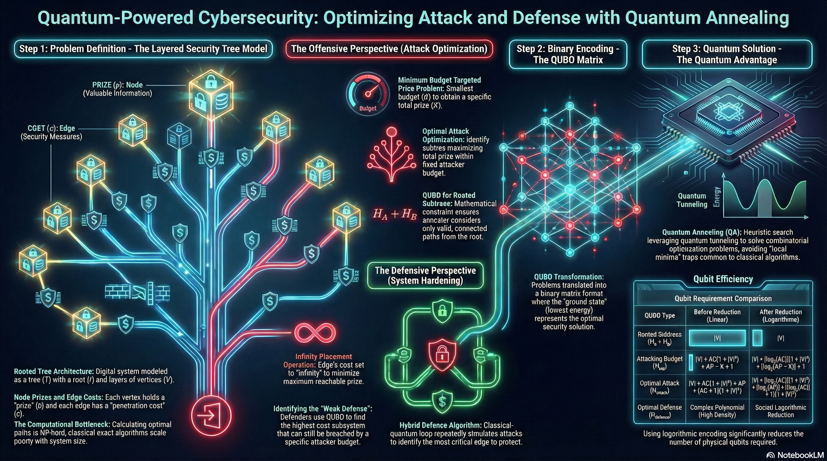
Executive Summary
This briefing examines the application of hybrid classical-quantum computation—specifically quantum annealing (QA)—to solve critical optimization problems within a layered cybersecurity framework. As digital interconnectedness increases, traditional classical methods often struggle with the NP-hard and coNP-hard complexities inherent in cybersecurity modeling.Recent research, published in The Journal of Supercomputing (July 2025), demonstrates that cybersecurity scenarios can be modeled as rooted tree structures where penetration costs and node “prizes” (assets) are analyzed through Quadratic Unconstrained Binary Optimization (QUBO) formulations. By leveraging quantum tunneling, these quantum-ready Hamiltonians can identify optimal attack strategies and defense configurations more effectively than classical simulated annealing.
Key takeaways include:
● Model Versatility: Cybersecurity is represented as a rooted tree $T = (V, E)$ , where edges represent penetration costs and nodes represent potential attacker gains.
● Offensive/Defensive Symmetry: QUBO formulations have been developed and mathematically proven for both identifying maximum-prize attacks and placing “infinite cost” (unbreakable) security measures to minimize system vulnerability.
● Hybrid Efficiency: While current quantum hardware faces logical qubit limitations, the introduction of log-based qubit reduction techniques and hybrid classical-quantum algorithms (such as the Infinity Placement Optimization) offers a viable path toward real-world implementation.
● Experimental Validation: Results from D-Wave simulators confirm that formulated Hamiltonians consistently converge on ground states representing optimal cybersecurity strategies.
1. The Rooted Tree Cybersecurity Model
The foundational framework for this analysis is a layered security model where the system is viewed as a graph, specifically a rooted tree.
● Cybersecurity Model ( $M$ ): Defined as a three-tuple $M = (C, P, T)$ , where $T$ is a tree rooted at $r$ .
● Penetration Costs ( $C$ ): Assigned to the edges $E(T)$ . These represent the “budget” an attacker must spend to traverse a layer.
● Prizes ( $P$ ): Assigned to the non-root vertices $V(T)$ . These represent the value of the information or assets located at that node.
● System Attack: Modeled as a subtree $\tau$ containing the root $r$ . The attacker’s goal is to maximize the sum of prizes $pr(p, \tau)$ while ensuring the total cost $cst(c, \tau)$ does not exceed their budget $B$ .
Complexity Challenges
Solving these problems exactly is computationally intensive. The Optimal Attack Optimization Problem is proven to be NP-hard, while the Infinity Placement Optimization Problem (placing the strongest defense) is coNP-hard. Classical exact algorithms scale at $O(G^2n)$ or $O(G^2n^2)$ , where $G$ is the total prize value.
2. Quantum Annealing Methodology
Quantum Annealing (QA) addresses these optimization problems by transforming them into the task of finding a minimum energy configuration (ground state) of a physical system.
Core Principles
● Adiabatic Evolution: The system transitions from an initial Hamiltonian ( $H_I$ ), where the ground state is easy to identify, to a problem Hamiltonian ( $H_F$ ), which encodes the cybersecurity objective.
● Quantum Tunneling: Unlike classical simulated annealing, which must “climb” over energy barriers, QA allows the system to tunnel through them, potentially finding the global minimum in complex landscapes where classical algorithms become trapped.
● QUBO Formulation: The problems are converted into Quadratic Unconstrained Binary Optimization (QUBO) form, which is compatible with current quantum hardware like D-Wave annealers.
3. Offensive Strategies: Attack Formulations
The research identifies two primary offensive optimization problems and provides verified QUBO constructions for each.
3.1. Minimum Budget Targeted Prize Problem
An attacker seeks to determine the lowest budget $B$ required to obtain a total prize value of at least $K$ .
● QUBO Solution ( $H_{MB}$ ): This Hamiltonian penalizes configurations that do not form a valid rooted subtree or fail to reach the target prize $K$ . It uses a penalty constant $L > c_{max}|E(T)|$ to ensure the budget is minimized only after prize constraints are met.
3.2. Optimal Attack Optimization Problem
Given a fixed budget $B$ , the attacker seeks to maximize the prize collected.
● QUBO Solution ( $H_{attack}$ ): This formulation transforms a maximization problem into a minimization one by using a negative prize sum.
● Theorem 2: $H_{attack}$ yields $-1 \times$ an optimal solution to the maximum prize problem at the end of the ideal annealing process.
4. Defensive Strategies: System Protection
Defense focuses on identifying system weaknesses and deploying “infinite cost” measures—security protections that completely prevent access (e.g., hardware-level isolation or unbreakable encryption).
4.1. Weak Defense Identification
The Weak Defense Problem identifies the subsystem with the highest cost that remains attackable within a specific budget $B$ . This allows defenders to know where to avoid placing expensive assets.
● QUBO Solution ( $H_W$ ): Identifies the rooted subtree with the maximum edge cost sum that is $\leq B$ .
4.2. Optimal Defense (Infinity Placement)
This problem seeks to find exactly one edge to protect with an “infinite” cost to minimize the maximum prize an attacker could obtain.
● Hybrid Algorithm: Because this involves a “min-max” operation (minimizing the maximum prize), it utilizes a hybrid classical-quantum approach.
● Mechanism: It iteratively tests different placements of infinity using $H_{defense}$ and a threshold $U$ . The algorithm removes non-optimal placements until the best defense edge is identified.
5. Technical Optimization and Qubit Efficiency
To make these Hamiltonians practical for current quantum hardware, several transformation techniques are utilized:
5.1. Polynomial Reduction
Non-quadratic higher-degree polynomials (terms with 3 or more variables) are reduced to QUBO format using ancillary binary variables.
● If $a < 0$ : $as_iq_uq_v = aw(s_i + q_u + q_v – 2)$
● If $a > 0$ : $as_iq_uq_v = a\{w(s_i + q_u + q_v – 1) + (s_iq_u + q_uq_v + q_vs_i) – (s_i + q_u + q_v) + 1\}$
5.2. Qubit Reduction (Logarithmic Encoding)
Instead of using $N$ binary variables to encode values $1, \dots, N$ , the researchers employ a log-encoding trick:
● Only $m+1$ binary variables are required, where $m = \lfloor \log_2 N \rfloor$ .
● This significantly reduces the logical qubit footprint for variables representing total prizes ( $AP$ ) and total costs ( $AC$ ).| QUBO Type | Before Reduction Qubits | After
Reduction Qubits || —— | —— | —— || $H_A + H_B$ | $ | V || $H_W$ | $ | V || $H_{attack}$ | High Dependency on $AP, AC$ | Significantly reduced via $\lfloor \log_2 \rfloor$ |
6. Experimental Validation
Theoretical findings were supported by experiments using the D-Wave Ocean SDK and ExactSolver .
● Subtree Generation: Experiments successfully generated all possible rooted subtrees for various test graphs, proving that the constraints $H_A + H_B = 0$ effectively filter out invalid (disconnected) subtrees.
● Budgeting and Attacks: Tested scenarios (e.g., Tree 1 with $K=8$ ) correctly identified minimum budgets (Energy -645 + Offset 650 = 5) and maximum prizes within specific budgets.
● Weak Defense: For a budget of $B=5$ on a sample tree, the solver correctly identified the highest-cost attackable subsystem (Cost 5).
● Infinity Placement: The $H_{\infty}$ constraint was validated to ensure that exactly one placement of the strongest security measure was selected during the defense optimization process.
7. Strategic Conclusions and Practical Relevance
The research establishes that while quantum hardware is still maturing, the theoretical and experimental groundwork for quantum-assisted cybersecurity is robust.
Key Insights
● Real-Life Application: Trees represent actual layered security networks. Experts can assign prizes (asset values) and penetration costs (measure effectiveness) to run these models on quantum annealers to derive optimal strategies.
● The “Speedup” Debate: While researchers note that QA may not provide an exponential speedup for NP-complete problems compared to all classical methods, “the coefficients $\alpha$ and $\beta$ may be smaller than those of known classical algorithms.”
● Current Limitations: The primary hurdle is the number of logical qubits required. Complex constraints increase embedding size, and current hardware is not yet ready for massive, real-world intrusion detection datasets.
● Scaling: In practice, large cost/prize values can be scaled down for the annealer and scaled back up post-process to maintain accuracy within hardware limits.”Quantum annealing represents a promising complementary tool for enhancing cybersecurity in the quantum era,” offering superior solution quality through its unique ability to navigate complex energy landscapes.
SYNTHESIS OF EXPERIMENTAL APPARATUS AND METHODS FOR 1D SINGLE-ATOM ARRAYS
http://rcqt.science.cmu.ac.th/wp-content/uploads/2026/22Experimental apparatus and methods – Eng.png
Executive Summary
This document synthesizes the experimental designs and methodologies for the synthesis of a one-dimensional (1D) single-atom array using rubidium-85. The research identifies a shift in the field of neutral atom quantum computing from probabilistic single-atom preparation to more accessible methods involving vacancy determination and atom rearrangement for defect-free arrays.
Key takeaways include:
● Infrastructure: A robust ultra-high vacuum system was established, reaching pressures as low as $9 \times 10^{-11}$ mbar, crucial for prolonging single-atom lifetime.
● Cooling and Trapping: A six-beam Magneto-Optical Trap (MOT) successfully cooled rubidium-85 atoms to $94 \mu \text{K}$ , a temperature significantly below the Doppler cooling limit ( $140 \mu \text{K}$ ), attributed to polarization gradient cooling.
● Array Synthesis: Using a programmable Acousto-Optic Deflector (AOD) driven by software-defined radio, the researchers created a 1D array of five identical optical dipole traps with a $4 \mu \text{m}$ separation and $1 \mu \text{m}$ beam waist.
● Optimization: Individual control over the power and phase of multi-tone RF frequencies was utilized to homogenize trap amplitudes, overcoming interference distortions.
● Current Limitations: While the system can trap approximately 35 atoms per dipole trap, single-atom resolution remains unresolvable due to stray light and laser power fluctuations. Future improvements involve transitioning to 2D arrays via Spatial Light Modulators (SLM) and scaling to 100 traps.
1. Experimental Infrastructure and Vacuum Systems
The foundational requirement for maintaining a single-atom array is a vacuum environment that minimizes scattering with room-temperature background gases.
● Vacuum Assembly: The system utilizes a borosilicate glass cell ( $30 \times 30 \times 100 \text{ mm}$ ) integrated with a 10 l/s ion pump and a 150 l/s ion pump.
● Pressure Management: Following a 2-day bake-out at 180° Celsius, the system achieved a settled pressure of approximately $9 \times 10^{-11}$ mbar.
● Magnetic Control: Two coil sets surround the glass cell:
● Circular Anti-Helmholtz Coils: 150 turns per coil, generating the gradient required for the MOT.
● 3-axis Cube Helmholtz Coils: Used to relocate the zero magnetic field position through a central uniform field.
2. Magneto-Optical Trap (MOT) Configuration
The MOT serves as the primary cooling stage before atoms are loaded into the optical dipole traps.
2.1 Laser Systems and Frequency Locking
The setup utilizes two primary laser paths:
● Cooling Laser: A MOGLabs cateye diode laser (70.0 mW) amplified via a tapered chip to 600 mW. It is frequency-locked on the $5S_{1/2}, F = 3 \rightarrow 5P_{3/2}, F = 3co4$ transition, with a detuning range of -52 MHz to -4 MHz.
● Repumping Laser: A self-made ECDL producing 90.0 mW, frequency-locked on the $5S_{1/2}, F = 2 \rightarrow 5P_{3/2}, F = 2co3$ transition (detuned +8.6 MHz).
2.2 Beam Alignment
The system employs a retroreflective six-beam MOT configuration. Due to geometric restrictions, beams on the xy-plane intersect at a 60-degree angle. The beams are combined via polarization beam splitters (PBS), expanded to 8 mm diameters, and converted to $\sigma^+$ polarization using quarter-wave plates before entering the glass cell.
3. Optical Dipole Trap (ODT) Array Synthesis
The transition from a cloud of cooled atoms to a structured array is achieved through an optical dipole trap setup.
3.1 Array Generation via AOD
The ODT uses an 840 nm diode laser (650 mW). The beam is processed through:
● Acousto-Optic Deflector (AOD): Driven by multi-tone RF frequencies generated by a software-defined radio (Ettus USRP X310).
● RF Control: The frequencies (96, 98, 100, 102, and 104 MHz) radially spread the beam into five rays.
● Optical Path: A 4f system consisting of two 300 mm focal length lenses, followed by a dichroic mirror and a 50X objective lens, focuses the beams into the glass cell.
3.2 Power Homogenization
Interference between RF frequencies in the AOD can cause non-homogeneous trap power. By independently adjusting the frequency, amplitude, and phase of each RF tone, researchers successfully optimized the array to produce uniform trap amplitudes.Table: Optical Dipole Trap Specifications | Feature | Value | | :— | :— | | Beam Waist | $1 \mu \text{m}$ (focused) / $4 \mu \text{m}$ (for loading) | | Trap Separation | $4 \mu \text{m}$ | | Trap Depth ( $U_0$ ) | $h \times (-23) \text{ MHz} \approx k_B \times 1.1 \text{ mK}$ | | Total Max Power | 50 mW |
4. Performance Metrics and Results
4.1 MOT Characteristics
The MOT was evaluated using fluorescence signals and thermal expansion relations (release and recapture method).
● Atom Number: $1.10 \times 10^8$ .
● Density: $1.79 \times 10^{11} \text{ cm}^{-3}$ .
● Temperature: $94 \mu \text{K}$ .
● Note: This is significantly lower than the $140 \mu \text{K}$ Doppler limit for rubidium-85, likely due to polarization gradient cooling from the repumping beams.
● Magnetic Gradients: 24.3 G/cm (axial) and 13.8 G/cm (radial).
4.2 Atom Loading to ODT
Atoms are transferred to the ODT following a specific timing sequence:
Loading: MOT coils and cooling/repumping beams are active for 1 second.
Transition: MOT coils are deactivated for 10 ms.
Imaging: A 50 ms fluorescence imaging pulse is applied.Currently, this process yields an average of 35 atoms per trap . The loading distribution is broad, and single-atom resolution is not yet achieved.
5. Limitations and Technical Scope for Improvement
The document identifies several barriers to achieving a defect-free, scalable single-atom array and proposes specific technical solutions:
● Imaging Quality: Current imaging uses the MOT beam, leading to high background stray light. Solution: Implement a small-diameter retro-reflected imaging beam separate from the MOT beam and utilize 780 nm narrow bandpass filters.
● Single-Atom Resolution: Loading is currently not in the “collisional blockade” regime. Solution: Optimize loading parameters to enter this regime, which increases the probability of trapping exactly one atom.
● Stability: Fluctuations in laser power affect MOT density. Solution: Integration of an active laser power stabilizer.
● Scalability:
● Trap Quantity: Currently limited to 10 traps by 840 nm laser power. Upgrading to a higher power laser could increase this to 100 traps (the bandwidth limit of the AOD).
● Dimensionality: 1D arrays offer limited application variety. Solution: Transition to a 2D trap array using a Spatial Light Modulator (SLM).
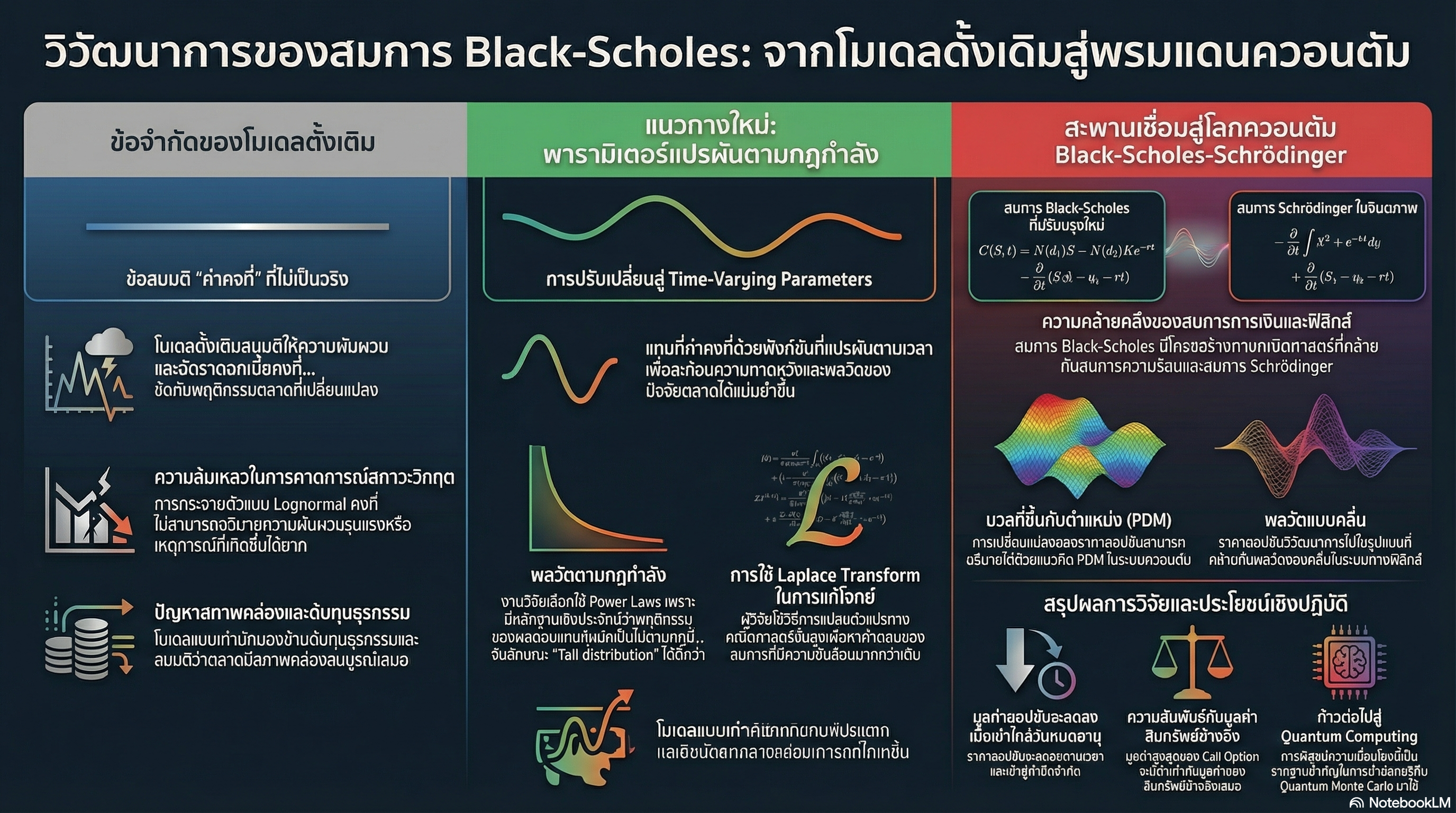
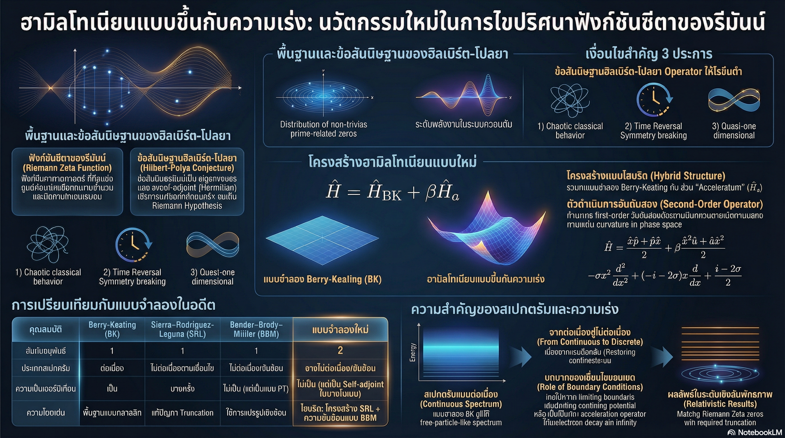
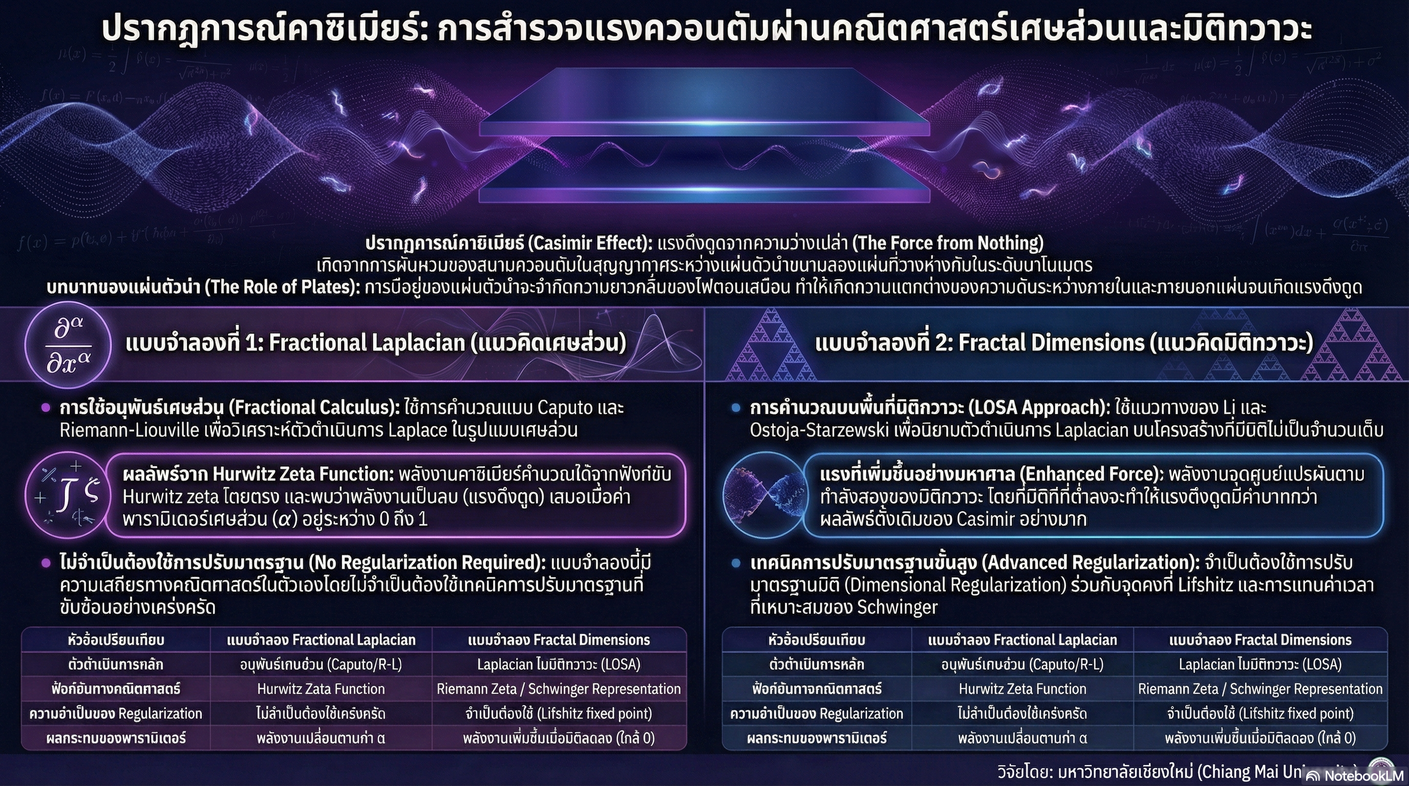
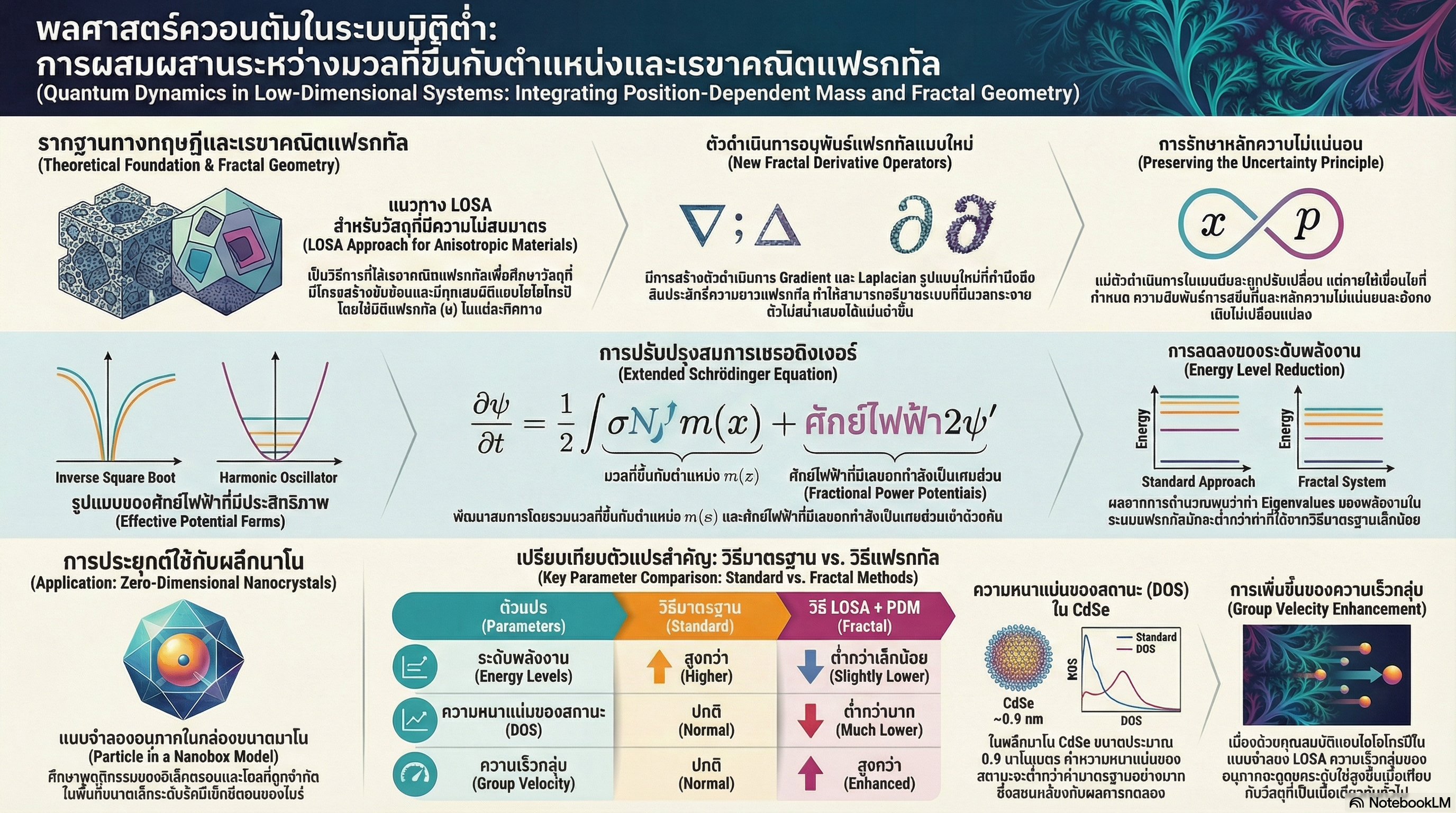
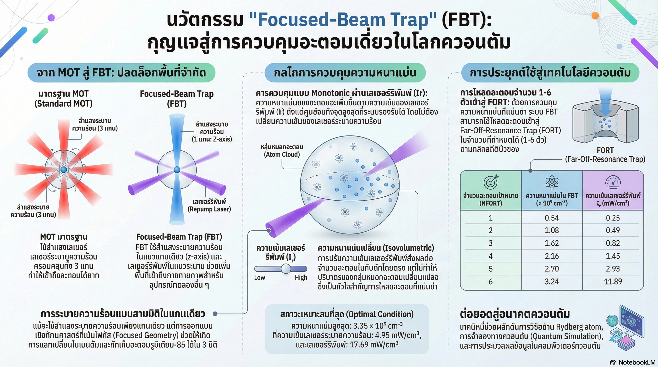
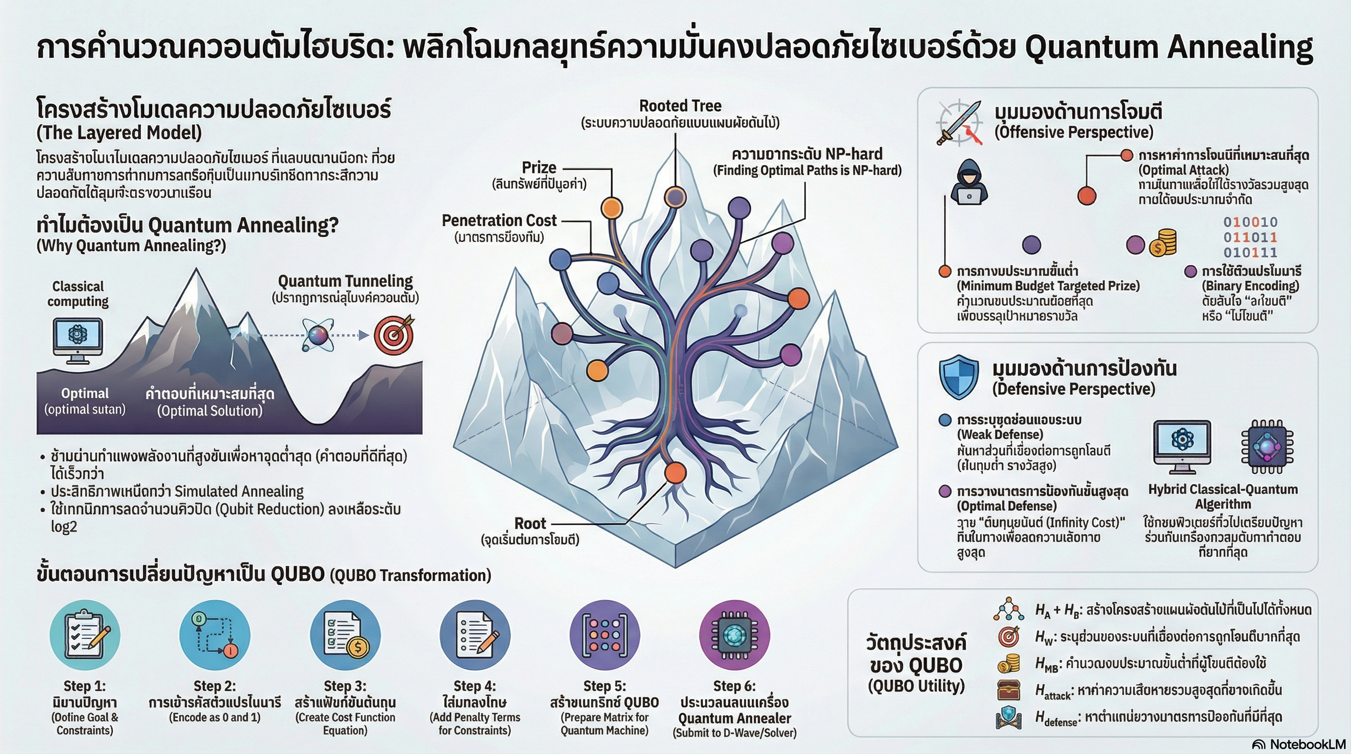